REVIEW 3 major objections 6 minor 55 references
The ExoTETHyS package: Tools for Exoplanetary Transits around Host Stars
T0 review · 3 major / 6 minor · reviewed 2026-08-14 · deepseek-v4-flash
Pith's one-line read ExoTETHyS fits stellar limb darkening so precisely that its model transit light curves reproduce exact reference calculations to better than 10 parts per million at every wavelength.
desk verdict Solid software paper with a credible few-ppm limb-darkening fitting method; the headline precision claim is broadly right but needs a caveat about the numerical reference and a single test case. read the letter →
The pith
A machine-rendered reading of the paper's core claim, the machinery that carries it, and where it could break.
The reading
What carries the argument
The central object is the weighted-r quasi-spherical (QS) fit: a weighted least-squares fit of an analytic limb-darkening law to a passband-integrated stellar intensity profile, with weights proportional to the radial sampling interval in $r = \sqrt{1-\mu^2}$ and a cutoff discarding intensities at $r > 0.99623$. The cutoff removes the steep limb drop-off characteristic of spherical model atmospheres, which has negligible effect on the numerically integrated light curve but distorts the coefficient fit; the weights ensure the fit prioritizes the radial intervals that actually contribute to the flux integral. The procedure also rescales spherical intensity profiles to the photometric radius defined by the inflection point of the intensity gradient, so the cutoff applies uniformly across models. This fitting method, implemented in the SAIL subpackage, is what carries the sub-10 ppm precision claim; the companion TRIP subpackage generates reference light curves by direct numerical integration of the occulted flux without any limb-darkening approximation.
What would settle it
Generate a noiseless reference transit light curve with TRIP using an intensity profile from an independent stellar atmosphere code not in ExoTETHyS's grids (e.g., a 3D or MESA model) for a star like HD 209458; if claret-4 coefficients from the weighted-r QS fit reproduce that curve with residuals above about 10 ppm, the claimed precision is specific to the grid rather than general.
Extended reading notes
Core claim
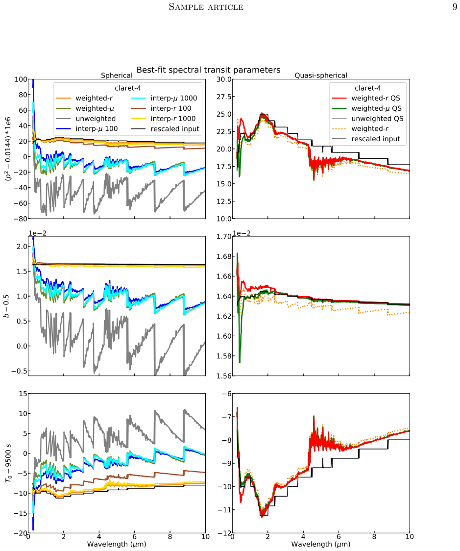
The central discovery is that the choice of fitting algorithm for limb-darkening coefficients, not just the choice of limb-darkening law or stellar atmosphere model, controls the accuracy of transit light-curve models at the tens-of-ppm level, and that a weighted least-squares fit with weights proportional to the sampling interval in the radial coordinate $r$, combined with a cut at $r \leq 0.99623$ to discard the steep intensity drop-off of spherical models, is the optimal procedure. With the claret-4 law, this weighted-r QS method reproduces noiseless reference light curves generated by direct numerical integration (TRIP) with peak-to-peak residuals of 2 ppm and rms below 1 ppm in the TESS passband, and below 8 ppm across 0.25–10 µm. The same coefficients retrieve the correct transit depth within 5 ppm, impact parameter within $6 \times 10^{-4}$, and transit duration within 1 s at all wavelengths. The paper concludes that claret-4 coefficients obtained through this algorithm ensure a precision of less than or about 10 ppm in relevant transit light curves at all wavelengths, exceeding by one order of magnitude the precision of most previously proposed algorithms for spherical stellar models.
Load-bearing premise
The validation is an internal consistency check: reference light curves are produced by TRIP from the same model-atmosphere intensity profiles to which the limb-darkening laws are fitted, so the claimed precision holds only if those atmosphere models (ATLAS, PHOENIX) represent real stellar surfaces.
Editorial extensions
If this is right
- For any transit modeled with claret-4 coefficients from SAIL, the systematic error contributed by limb-darkening parameterization is below about 10 ppm at all wavelengths, so it will sit under the expected photon noise of TESS, JWST, and ARIEL observations for typical targets.
- Two-coefficient laws (quadratic, power-2, square-root) are shown to be unreliable below 1 µm for exoplanet spectroscopy, introducing biases of tens to hundreds of ppm, so the claret-4 law must be preferred at optical and ultraviolet wavelengths.
- The proposed formula $(\text{peak-to-peak})_{\mathrm{ppm}} = (k \times 10^6) \times p^2 \times (\text{weighted-r QS rms})$ lets users estimate the systematic noise floor of their light-curve model from the intensity-fit residuals alone, allowing a quick check that limb-darkening systematics stay below the photon-noise limit.
- Because the algorithm eliminates the degeneracy among previous fitting methods (unweighted, weighted-μ, interpolated-μ/r, and their QS variants), different analyses of the same star and passband will obtain identical limb-darkening coefficients and hence mutually consistent transit parameters.
Reading between the lines
- The paper validates precision against internally generated light curves; a natural extension is to test the same weighted-r QS coefficients against real ultra-precise space photometry (e.g., TESS or JWST) for stars with well-determined parameters, where residuals below about 10 ppm would corroborate the accuracy claim.
- Because the QS cutoff at $r \leq 0.99623$ is defined on the rescaled photometric radius, the method may be more robust than the original $\mu \geq 0.1$ cutoff for giant and supergiant stars whose intensity drop-off occurs at larger $\mu$; one could quantify the coefficient bias for low-gravity PHOENIX models to test this.
- Equation (20) suggests a cheap, instrument-independent quality metric: a user comparing any two limb-darkening laws or algorithms can predict the resulting light-curve bias without running full transit fits, and this could be extended to choose the minimal polynomial degree needed to reach a target precision for a given passband and star.
- The TRIP exact integrator, being free of limb-darkening approximations, is the natural tool to assess biases in other transit parameters beyond depth; the paper's parameter-recovery tests for HD 209458b hint that these biases are sub-ppm in the QS case, but the same check could be run for grazing transits or small planets where the limb contribution is relatively larger.
Signed reviews
Editorial analysis
A structured set of objections, weighed in public.
Referee Report
Summary. The paper introduces ExoTETHyS, an open-source Python package with two subpackages. SAIL computes stellar limb-darkening coefficients by fitting parametric limb-darkening laws to passband-integrated model-atmosphere intensity profiles, using a weighted-r least-squares fit with a quasi-spherical cutoff (weighted-r QS). TRIP generates transit light curves by direct numerical integration of the full stellar intensity profile rather than through limb-darkening coefficients. The authors validate SAIL by generating noiseless reference light curves with TRIP from PHOENIX and ATLAS intensity profiles for an HD209458b-like system, then fitting those light curves with models that use coefficient sets obtained by different fitting methods and limb-darkening laws. They report that claret-4 coefficients from the weighted-r QS method reproduce the reference TESS light curve to 2 ppm peak-to-peak and the spectral light curves (20 nm bins over 0.25-10 micron) to below 8 ppm peak-to-peak, and they propose Eq. (20) to predict light-curve residuals from the intensity-profile fit residual. The central claim is that this algorithm outperforms most previously proposed fitting algorithms by about an order of magnitude for spherical stellar models.
Significance. If the headline precision claim is sustained, ExoTETHyS is a genuinely useful tool for high-precision transit spectroscopy, particularly for JWST and ARIEL simulations and data analysis. The paper's strengths include the release of reproducible, documented code; a direct-integration transit generator (TRIP) that sidesteps limb-darkening parameterizations entirely; and a validation strategy that correctly isolates the limb-darkening parameterization error: reference light curves and fitted coefficients both derive from the same model intensity profile, so the residuals measure how well a given parametric law reproduces the exact integral. This internal-consistency test is not circular for the paper's stated purpose, and the paper explicitly disclaims empirical validation against real stellar surfaces. The comparison of fitting methods is also useful and will help practitioners choose among algorithms. However, the generality of the <10 ppm claim rests on a single test geometry and a single stellar model, and the numerical accuracy of the TRIP reference is not demonstrated, so the strongest headline statements are not yet fully supported.
major comments (3)
- [Section 2.2.3 and Section 3.1] The central precision claim is measured against reference light curves generated by TRIP, but the numerical accuracy of TRIP itself is not established. Equations (16) and (17) are evaluated with the midpoint rule on a uniform partition in r, yet the paper gives no default annulus count, no convergence study, and no independent check against an analytic or high-accuracy reference. If TRIP's own discretization error is comparable to 1-10 ppm, then the reported 2 ppm TESS residual and <8 ppm spectral residuals are not a clean measurement of the limb-darkening approximation error. The authors should state the default number of annuli, demonstrate convergence with respect to that parameter, and, ideally, validate TRIP against an independent integrator or an analytic solution.
- [Section 3.1, Section 3.3, and Table 1] The headline '<10 ppm at all wavelengths' is established from one HD209458-like PHOENIX 2012 stellar model and one transit geometry. Equation (20) explicitly introduces a p^2 dependence, and the residual magnitude should also depend on impact parameter and the stellar intensity profile, but no tests are shown over the Teff, log g, [M/H], p, or b ranges covered by the package grids in Table 1. The cutoff r <= 0.99623 is also a free choice, and no sensitivity to that cutoff is reported. The validation should be extended, or the claims should be explicitly restricted to the tested regime, before stating that the algorithm ensures <10 ppm precision for relevant transit light curves generally.
- [Abstract and Section 5] The statement that the algorithm outperforms 'most of the algorithms proposed in the previous literature' by one order of magnitude is not uniformly supported by the paper's own Figures 2 and 3. For the TESS simulation, weighted-mu QS and unweighted QS give peak-to-peak residuals of 3 ppm, only marginally worse than the 2 ppm of weighted-r QS, and the spectral residuals of the other QS methods remain below 13 ppm rather than a factor of ten larger. The order-of-magnitude improvement is persuasive relative to unweighted spherical fits, but the sweeping wording should be tightened to specify the comparison class and to acknowledge that the advantage over other quasi-spherical fits is modest in the tested case.
minor comments (6)
- [Section 2.1.3, Eq. (6)] In Eq. (6), the summation index is k but the coefficient is written as a_n; this should be a_k (or the index should be n).
- [Section 2.1.1] The text contains a typo: 'whic includes' should be 'which includes'.
- [Section 3.1, bottom of page 8] The sentence describing interp-r residuals says 'about 1.5 and 2 times larger residual amplitudes, respectively'; the pairing of the two interpolation grids with the two factors is ambiguous and should be clarified.
- [Section 3.3 and Figure 5 caption] Section 3.3 refers to 'HD20458 b' while the rest of the paper uses HD209458 b; the Figure 5 caption contains a similar typo ('HD20458 b').
- [Section 2.1.4] The value r_cut = 0.99623 is stated without explanation of where it comes from; a sentence explaining the origin of the numerical value and its precision would help users judge the robustness of the quasi-spherical cutoff.
- [Section 3.3, Eq. (20)] Equation (20) introduces a free factor k with k approximately 1, but the paper does not give the fitted values of k obtained in the 'different transit parameters' tests or specify the range of geometries over which the proportionality was checked; providing this information would make the formula more actionable.
Circularity Check
No significant circularity: the <10 ppm claim is a forward-model approximation test, not a fitted-input prediction.
full rationale
The paper's central precision claim is established by comparing transit light curves computed from fitted limb-darkening coefficients against reference light curves generated by direct numerical integration of the same model intensity profiles. This is an internal consistency test of how well the claret-4 parametric law approximates the exact integral; it is not a reduction to the fitted inputs. The coefficients are fitted to the intensity profiles via the weighted-r QS algorithm (Equations 9-10), while the reference light curves are produced independently by TRIP from the same intensity profiles (Equations 16-19). No coefficient is fitted to the reference light curves, and no transit parameter is predicted from a fitted value. The weighted-r QS method is one of several discrete fitting algorithms compared, not a parameter fitted to the validation light curves, so the reported ranking is not forced by construction. The paper explicitly limits its claim to model precision and acknowledges the lack of empirical validation: 'the lack of empirical validation for stellar limb-darkening prevents the final choice of the most reliable model(s)', and Equation 20 'does not account for uncertainties in the stellar parameters, discrepancies between real and model intensity profiles, and other contaminating signals'. Self-citations, such as the TRIP algorithm being identical to the 'tlc' of Morello et al. (2017), are references to fully specified numerical methods, not load-bearing circular premises. No circular step can be exhibited from the paper's equations or claims.
Assumptions & free parameters
free parameters (2)
- r_cut =
0.99623
- k =
order unity (~1)
assumptions (4)
- domain assumption ATLAS and PHOENIX model atmosphere intensity profiles are treated as ground truth for the accuracy tests.
- domain assumption The star is spherically symmetric and unspotted, and the planet is a dark sphere.
- domain assumption The photometric radius is defined as the inflection point of the intensity profile, with radial coordinates rescaled so this radius is r=1.
- domain assumption The TRIP numerical integration of the model intensity profile is exact enough that residuals isolate the limb-darkening law approximation error.
Cite this review
Pith. "Pith review of The ExoTETHyS package: Tools for Exoplanetary Transits around Host Stars." pith.science (2026). https://pith.science/paper/LXEAKK4F
@misc{pith2026190809599,
  author       = {Pith},
  title        = {Pith review of: The ExoTETHyS package: Tools for Exoplanetary Transits around Host Stars},
  year         = {2026},
  howpublished = {\url{https://pith.science/paper/LXEAKK4F}},
  note         = {Machine review of arXiv:1908.09599}
}
read the original abstract
We present here the first release of the open-source python package ExoTETHyS, which aims to provide a stand-alone set of tools for modeling spectro-photometric observations of the transiting exoplanets. In particular, we describe: (1) a new calculator of stellar limb-darkening coefficients that outperforms the existing software by one order of magnitude in terms of light-curve model accuracy, i.e., down to <10 parts per million (ppm); (2) an exact transit light-curve generator based on the entire stellar intensity profile rather than limb-darkening coefficients. New tools will be added in later releases to model various effects in exoplanetary transits and eclipsing binaries. ExoTETHyS is a reference package for high-precision exoplanet atmospheric spectroscopy with the upcoming JWST and ARIEL missions.
Figures


Figures from the paper (3 more)


Reference graph
Works this paper leans on
-
[1]
Analytic Planetary Transit Light Curves and Derivatives for Stars with Polynomial Limb Darkening
Agol, E., Luger, R., & Foreman-Mackey, D. 2019, arXiv e-prints, arXiv:1908.03222. https://arxiv.org/abs/1908.03222
work page Pith review arXiv 2019
-
[2]
Akinsanmi, B., Barros, S. C. C., Santos, N. C., et al. 2019, A&A, 621, A117, doi: 10.1051/0004-6361/201834215
-
[3]
Ballerini, P., Micela, G., Lanza, A. F., & Pagano, I. 2012, A&A, 539, A140, doi: 10.1051/0004-6361/201117102
-
[4]
W., Linscott, E., & Shporer, A
Barnes, J. W., Linscott, E., & Shporer, A. 2011, ApJS, 197, 10, doi: 10.1088/0067-0049/197/1/10
-
[5]
2014, PASP, 126, 1134, doi: 10.1086/679566
Beichman, C., Benneke, B., Knutson, H., et al. 2014, PASP, 126, 1134, doi: 10.1086/679566
doi:10.1086/679566 2014
-
[6]
2017, A&A, 597, A94, doi: 10.1051/0004-6361/201528018
Chiavassa, A., Caldas, A., Selsis, F., et al. 2017, A&A, 597, A94, doi: 10.1051/0004-6361/201528018
-
[7]
Christiansen, J. L., Jenkins, J. M., Caldwell, D. A., et al. 2012, PASP, 124, 1279, doi: 10.1086/668847
doi:10.1086/668847 2012
-
[8]
Claret, A. 2000, A&A, 363, 1081 —. 2003, A&A, 401, 657, doi: 10.1051/0004-6361:20030142 —. 2004, A&A, 428, 1001, doi: 10.1051/0004-6361:20041673 —. 2008, A&A, 482, 259, doi: 10.1051/0004-6361:200809370 —. 2017, A&A, 600, A30, doi: 10.1051/0004-6361/201629705 —. 2018, A&A, 618, A20, doi: 10.1051/0004-6361/201833060
Show all 55 references
-
[9]
2011, A&A, 529, A75, doi: 10.1051/0004-6361/201116451
Claret, A., & Bloemen, S. 2011, A&A, 529, A75, doi: 10.1051/0004-6361/201116451
2011 doi
-
[10]
2020, arXiv e-prints, arXiv:2001.07129
Claret, A., Cukanovaite, E., Burdge, K., et al. 2020, arXiv e-prints, arXiv:2001.07129. https://arxiv.org/abs/2001.07129
2020 arXiv
-
[11]
Claret, A., Dragomir, D., & Matthews, J. M. 2014, A&A, 567, A3, doi: 10.1051/0004-6361/201423515
2014 doi
-
[12]
H., & Witte, S
Claret, A., Hauschildt, P. H., & Witte, S. 2012, A&A, 546, A14, doi: 10.1051/0004-6361/201219849 —. 2013, A&A, 552, A16, doi: 10.1051/0004-6361/201220942
2012 doi
-
[13]
2013, A&A, 549, A9, doi: 10.1051/0004-6361/201219888
Csizmadia, S., Pasternacki, T., Dreyer, C., et al. 2013, A&A, 549, A9, doi: 10.1051/0004-6361/201219888
2013 doi
-
[14]
1992, A&A, 259, 227
Diaz-Cordoves, J., & Gimenez, A. 1992, A&A, 259, 227
1992
-
[15]
S., & Agol, E
Eastman, J., Gaudi, B. S., & Agol, E. 2013, PASP, 125, 83, doi: 10.1086/669497
2013 doi
-
[16]
2015, MNRAS, 450, 1879, doi: 10.1093/mnras/stv744 —
Espinoza, N., & Jord´ an, A. 2015, MNRAS, 450, 1879, doi: 10.1093/mnras/stv744 —. 2016, MNRAS, 457, 3573, doi: 10.1093/mnras/stw224
2015 doi
-
[17]
Z., Johnson, J
Gazak, J. Z., Johnson, J. A., Tonry, J., et al. 2012, Advances in Astronomy, 2012, 697967, doi: 10.1155/2012/697967 Gim´ enez, A. 2006, A&A, 450, 1231, doi: 10.1051/0004-6361:20054445
2012 doi
-
[18]
2019, ApJ, 878, 119, doi: 10.3847/1538-4357/ab2048 Hestroffer, D
Hellard, H., Csizmadia, S., Padovan, S., et al. 2019, ApJ, 878, 119, doi: 10.3847/1538-4357/ab2048 Hestroffer, D. 1997, A&A, 327, 199 Heyrovsk´ y, D. 2007, ApJ, 656, 483, doi: 10.1086/509566
2019 doi
-
[19]
Howarth, I. D. 2011a, MNRAS, 413, 1515, doi: 10.1111/j.1365-2966.2011.18122.x —. 2011b, MNRAS, 418, 1165, doi: 10.1111/j.1365-2966.2011.19568.x
2011
-
[20]
D., & Morello, G
Howarth, I. D., & Morello, G. 2017, MNRAS, 470, 932, doi: 10.1093/mnras/stx1260
2017 doi
-
[21]
G., & Benz, W
Isaak, K. G., & Benz, W. 2019, Nature Astronomy, 3, 873, doi: 10.1038/s41550-019-0886-9 Sample article 15
2019 doi
-
[22]
R., Swain, M
Iyer, A. R., Swain, M. R., Zellem, R. T., et al. 2016, ApJ, 823, 109, doi: 10.3847/0004-637X/823/2/109
2016 doi
-
[23]
M., & Tinetti, G
Kipping, D. M., & Tinetti, G. 2010, MNRAS, 407, 2589, doi: 10.1111/j.1365-2966.2010.17094.x
2010
-
[24]
1950, Harvard College Observatory Circular, 454, 1
Kopal, Z. 1950, Harvard College Observatory Circular, 454, 1
1950
-
[25]
2015, PASP, 127, 1161, doi: 10.1086/683602
Kreidberg, L. 2015, PASP, 127, 1161, doi: 10.1086/683602
2015 doi
-
[26]
2015, A&A, 573, A90, doi: 10.1051/0004-6361/201423804
Magic, Z., Chiavassa, A., Collet, R., & Asplund, M. 2015, A&A, 573, A90, doi: 10.1051/0004-6361/201423804
2015 doi
-
[27]
2002, ApJL, 580, L171, doi: 10.1086/345520
Mandel, K., & Agol, E. 2002, ApJL, 580, L171, doi: 10.1086/345520
2002 doi
-
[28]
2015, ApJ, 805, 28, doi: 10.1088/0004-637X/805/1/28
Masuda, K. 2015, ApJ, 805, 28, doi: 10.1088/0004-637X/805/1/28
2015 doi
-
[29]
Maxted, P. F. L. 2018, A&A, 616, A39, doi: 10.1051/0004-6361/201832944
2018 doi
-
[30]
2010, A&A, 521, L59, doi: 10.1051/0004-6361/201015550
Mazeh, T., & Faigler, S. 2010, A&A, 521, L59, doi: 10.1051/0004-6361/201015550
2010 doi
-
[31]
2012, A&A, 541, A56, doi: 10.1051/0004-6361/201117908
Mazeh, T., Nachmani, G., Sokol, G., Faigler, S., & Zucker, S. 2012, A&A, 541, A56, doi: 10.1051/0004-6361/201117908
2012 doi
-
[32]
2018, AJ, 156, 175, doi: 10.3847/1538-3881/aadda4
Morello, G. 2018, AJ, 156, 175, doi: 10.3847/1538-3881/aadda4
2018 doi
-
[33]
Lagage, P. O. 2019, AJ, 157, 205, doi: 10.3847/1538-3881/ab14e2
2019 doi
-
[34]
D., & Homeier, D
Morello, G., Tsiaras, A., Howarth, I. D., & Homeier, D. 2017, AJ, 154, 111, doi: 10.3847/1538-3881/aa8405
2017 doi
-
[35]
R., & Lester, J
Neilson, H. R., & Lester, J. B. 2013a, A&A, 554, A98, doi: 10.1051/0004-6361/201321502 —. 2013b, A&A, 556, A86, doi: 10.1051/0004-6361/201321888
-
[36]
B., Gizon, L., Cameron, R
Nielsen, M. B., Gizon, L., Cameron, R. H., & Miesch, M. 2019, A&A, 622, A85, doi: 10.1051/0004-6361/201834373
2019 doi
-
[37]
2015, MNRAS, 450, 3233, doi: 10.1093/mnras/stv894
Parviainen, H. 2015, MNRAS, 450, 3233, doi: 10.1093/mnras/stv894
2015 doi
-
[38]
2015, MNRAS, 453, 3821, doi: 10.1093/mnras/stv1857
Parviainen, H., & Aigrain, S. 2015, MNRAS, 453, 3821, doi: 10.1093/mnras/stv1857
2015 doi
-
[39]
2018, in Society of Photo-Optical Instrumentation Engineers (SPIE) Conference Series, Vol
Pascale, E., Bezawada, N., Barstow, J., et al. 2018, in Society of Photo-Optical Instrumentation Engineers (SPIE) Conference Series, Vol. 10698, Proc. SPIE, 106980H
2018
-
[40]
2014, Experimental Astronomy, 38, 249, doi: 10.1007/s10686-014-9383-4
Rauer, H., Catala, C., Aerts, C., et al. 2014, Experimental Astronomy, 38, 249, doi: 10.1007/s10686-014-9383-4
2014 doi
-
[41]
C., & Howarth, I
Reeve, D. C., & Howarth, I. D. 2016, MNRAS, 456, 1294, doi: 10.1093/mnras/stv2631
2016 doi
-
[42]
H., & Gizon, L
Reinhold, T., Cameron, R. H., & Gizon, L. 2017, A&A, 603, A52, doi: 10.1051/0004-6361/201730599
2017 doi
-
[43]
R., Winn, J
Ricker, G. R., Winn, J. N., Vanderspek, R., et al. 2014, in Society of Photo-Optical Instrumentation Engineers (SPIE) Conference Series, Vol. 9143, Proc. SPIE, 914320
2014
-
[44]
2016, in Society of Photo-Optical Instrumentation Engineers (SPIE) Conference Series, Vol
Sarkar, S., Papageorgiou, A., & Pascale, E. 2016, in Society of Photo-Optical Instrumentation Engineers (SPIE) Conference Series, Vol. 9904, Proc. SPIE, 99043R
2016
-
[45]
1906, Nachrichten von der Gesellschaft der Wissenschaften zu Gottingen, Mathematisch-Physikalische Klasse, 195, 43
Schwarzschild, K. 1906, Nachrichten von der Gesellschaft der Wissenschaften zu Gottingen, Mathematisch-Physikalische Klasse, 195, 43
1906
-
[46]
2003, ApJ, 585, 1038, doi: 10.1086/346105
Seager, S., & Mall´ en-Ornelas, G. 2003, ApJ, 585, 1038, doi: 10.1086/346105
2003 doi
-
[47]
2017, PASP, 129, 072001, doi: 10.1088/1538-3873/aa7112
Shporer, A. 2017, PASP, 129, 072001, doi: 10.1088/1538-3873/aa7112
2017 doi
-
[48]
Sing, D. K. 2010, A&A, 510, A21, doi: 10.1051/0004-6361/200913675
2010 doi
-
[49]
K., Fortney, J
Sing, D. K., Fortney, J. J., Nikolov, N., et al. 2016, Nature, 529, 59, doi: 10.1038/nature16068
2016 doi
-
[50]
2008, MNRAS, 386, 1644, doi: 10.1111/j.1365-2966.2008.13145.x
Southworth, J. 2008, MNRAS, 386, 1644, doi: 10.1111/j.1365-2966.2008.13145.x
2008
-
[51]
Southworth, J., Maxted, P. F. L., & Smalley, B. 2004, MNRAS, 351, 1277, doi: 10.1111/j.1365-2966.2004.07871.x
2004
-
[52]
P., Rocchetto, M., et al
Tsiaras, A., Waldmann, I. P., Rocchetto, M., et al. 2016, ApJ, 832, 202, doi: 10.3847/0004-637X/832/2/202
2016 doi
-
[53]
P., Zingales, T., et al
Tsiaras, A., Waldmann, I. P., Zingales, T., et al. 2018, AJ, 155, 156, doi: 10.3847/1538-3881/aaaf75
2018 doi
-
[54]
P., & Kervella, P
Wittkowski, M., Aufdenberg, J. P., & Kervella, P. 2004, A&A, 413, 711, doi: 10.1051/0004-6361:20034149
2004 doi
-
[55]
T., Swain, M
Zellem, R. T., Swain, M. R., Roudier, G., et al. 2017, ApJ, 844, 27, doi: 10.3847/1538-4357/aa79f5
2017 doi
Reviewed August 14, 2026 · model on record in the stance chip above.
Discussion (0). Continue with ORCID to comment.