REVIEW 4 major objections 4 minor 72 references
Boundedness of massless scalar waves on Kerr interior backgrounds
T0 review · 4 major / 4 minor · reviewed 2026-08-14 · deepseek-v4-flash
Pith's one-line read Massless scalar waves on every subextremal Kerr black hole are uniformly bounded up to the Cauchy horizon, to which they extend continuously.
desk verdict First boundedness result for scalar waves on the full subextremal Kerr interior; the proof architecture is credible, but the key blueshift positivity premise is asserted rather than proved—verifiable by direct computation and almost certainly true, so this is a fixable gap, not a fatal one. read the letter →
The pith
A machine-rendered reading of the paper's core claim, the machinery that carries it, and where it could break.
The reading
What carries the argument
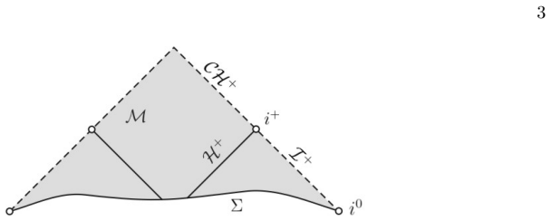
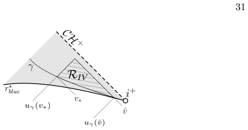
The engine is the vector-field method in Eddington–Finkelstein normalized double-null coordinates $(u,v,\theta_\star,\tilde\varphi)$, in which the metric takes the form $g=-2\Omega^2(du\otimes dv+dv\otimes du)+\cdots$. The interior is cut into redshift, noshift, and blueshift regions by the coordinate $r_\star$; the blueshift region is where the argument lives or dies. There the metric coefficient $\Omega^2$ decays exponentially along the characteristics, and the proof uses the weighted multiplier $S=|u|^p\partial_u+v^p\partial_v+v^p b_{\tilde\varphi}\partial_{\tilde\varphi}$ together with a spacelike hypersurface $\gamma$ that sits a logarithmic $v$-distance behind a constant-$r_\star$ hypersurface, chosen so that the integrated bulk and error terms become small. Commutation is by the standard angular momentum operators $Y_i$ ($i=1,2,3$; only $\partial_{\tilde\varphi}$ is Killing), and the final pointwise step is Sobolev embedding on the two-spheres $\mathbb{S}^2_{u,v}$, whose volume element differs from the round one by a bounded factor $L$. The positivity of the bulk term in the blueshift region rests on the asserted uniform lower bound on $-2\,\partial_\zeta\Omega/\Omega$ for $\zeta=u,v$.
What would settle it
Compute the quantity $-2\,\partial_\zeta\Omega/\Omega$ for $\zeta=u,v$ using the metric coefficient $\Omega^2=-\Delta/R^2$ throughout the interior for a grid of subextremal parameters, say $|a|/M=0.1,0.3,\dots,0.99$, and determine whether a threshold $r_\star^{\mathrm{blue}}$ exists such that both quantities are bounded below by a positive constant $\beta$ for all $r_\star\geq r_\star^{\mathrm{blue}}$. If for some allowed $a$ the quantity fails to have such a positive lower bound, the blueshift-region estimate (106) fails and the proof collapses.
Extended reading notes
Core claim
The central result, Theorem 1.1, claims that on subextremal Kerr spacetime with $M>|a|\neq 0$, any solution of $\Box_g\psi=0$ arising from sufficiently regular localized Cauchy data satisfies $|\psi|\leq C$ globally in the black hole interior, with $C$ explicitly computable from $a$, $M$, and a norm of the initial data, and that $\psi$ extends continuously to the bifurcate Cauchy horizon. The proof establishes the stronger weighted-energy statement of Theorem 1.2: for a weight exponent $p>1$ tied to the horizon decay rate, weighted fluxes of $\psi$ and its angular derivatives up to second order are finite all the way to the Cauchy horizon in a neighborhood of timelike infinity. Pointwise boundedness then follows by Sobolev embedding on the non-round spheres $\mathbb{S}^2_{u,v}$. The paper frames this as the Kerr analog of its earlier Reissner–Nordstr\"om result, with the new difficulty being the control of error terms produced by commuting with non-Killing angular momentum operators.
Load-bearing premise
The argument assumes that inside the blueshift region the metric coefficient $\Omega$ decays along the null directions at a rate uniformly bounded away from zero, for every subextremal rotation parameter, yet the paper only demonstrates this decay rate in the slow-rotation limit and otherwise invokes an analogy with the charged case.
Editorial extensions
If this is right
- Massless scalar fields never blow up on the Kerr Cauchy horizon for any subextremal rotation parameter, since the uniform bound $|\psi|\leq C$ holds up to and including $\mathcal{CH}^+$.
- Each solution extends continuously to the bifurcate Cauchy horizon, so well-defined limiting values of the field exist there rather than divergent or oscillatory behavior.
- The weighted energy bounds hold with polynomial weights $v^p$ and $|u|^p$ for $p>1$ up to the Cauchy horizon near timelike infinity, giving quantitative $L^2$ control on the field and its first two angular derivatives.
- The boundedness is global in the interior: combining the two ends near timelike infinity and invoking Cauchy stability on the remaining compact region covers the entire black hole interior.
- The result covers the full subextremal range $M>|a|\neq 0$, so it is not restricted to slow rotation.
Reading between the lines
- If Theorem 1.1 is correct, the Kerr Cauchy horizon is $C^0$-stable with respect to massless scalar waves for every subextremal spin; this is compatible with, not contradicted by, known instability results showing that non-degenerate energy generically blows up, because the theorem bounds $\psi$ itself rather than its derivatives.
- A direct analytic or numerical check of the asserted uniform lower bound on $-2\,\partial_\zeta\Omega/\Omega$ across the full range $|a|<M$ would settle the proof's main unproved input: a single parameter value where the lower bound fails would invalidate the result as stated.
- The same weighted-energy template, with the admissible weight tied to the exterior decay rate, suggests that faster exterior decay would permit heavier interior weights; whether an analogous hierarchy can be closed for gravitational perturbations is left open by this paper.
Signed reviews
Editorial analysis
A structured set of objections, weighed in public.
Referee Report
Summary. The paper proves Theorem 1.1: for a massless scalar wave on a fixed subextremal Kerr background with 0 < |a| < M, arising from sufficiently regular localized Cauchy data, the solution is uniformly bounded in the black hole interior up to and including the Cauchy horizon, to which it extends continuously. The proof is an extension of the author's Reissner–Nordström analysis [30]. It imports polynomial decay along the event horizon from [27], uses the geometry and metric estimates of Dafermos–Luk [19], and combines a redshift vector field near H+, a noshift argument in the intermediate region, and a blueshift analysis near CH+. The blueshift part distinguishes a hypersurface γ of logarithmic distance from r* = r*_blue, uses a weighted multiplier S0 before γ and S = |u|^p ∂u + v^p(∂v + b̃φ ∂φ̃) after γ, controls error terms from commutation with angular momentum operators, and derives pointwise bounds via Sobolev embedding on the spheres.
Significance. If the proof is completed as intended, this is a significant result: it would establish uniform boundedness of scalar waves at the Kerr Cauchy horizon for the full subextremal range, without symmetry assumptions, complementing the instability results of Luk–Sbierski (infinite non-degenerate energy) and the C0 stability of Dafermos–Luk for the vacuum equations. The paper is careful to rely on independent exterior decay results and geometric bounds, and the constant in Theorem 1.1 is explicit in terms of the data; there is no circularity in the central argument. The main weaknesses are that several load-bearing estimates in the blueshift region are only sketched, and one displayed absorption estimate (Lemmas 4.14 and 4.19) appears to pair terms with the wrong flux components as written.
major comments (4)
- [§4.4.2 (Eqs. (169)–(172))] The absorption argument in Lemma 4.14 is not internally consistent as written: the first line of K̃_S in (169) contains |u|^p(∂uψ)^2/(2Ω²), which is naturally bounded by the v = const flux JS_μ n^μ_{v=const} in (156), while (171) bounds it by JS_μ n^μ_{u=const} in (157); the second line is mismatched in the opposite way. As a result, the displayed estimate (172) does not follow from (171), and the smallness of δ1 and δ2 is not established. The same pattern appears for the W-multiplier in §4.6, equations (196)–(200). Since Proposition 4.15 and hence Theorem 4.18 depend on Lemma 4.14, this needs to be carefully rewritten.
- [§4.4.2 (Eqs. (168), (173)–(174))] The Cauchy–Schwarz treatment of the ∂u b̃φ cross terms is too compressed. The estimate (168) produces a term with coefficient v^p √(∂u b̃φ)/(4Ω²) multiplying (∂vψ)^2; when this is incorporated into K̃_S in (169), the subsequent bounds (173)–(174) replace √(∂u b̃φ) by a pointwise decaying quantity, but after the division by Ω² that is explicit in (169) an extra factor Ω^{-1} remains. The authors must show how this factor is absorbed by the corresponding boundary flux before claiming the stated smallness. As written, the displayed estimates do not justify the claimed δ1 and δ2 rates.
- [§2.2.7 (Eq. (106))] The lower bound (106) is asserted for the whole subextremal range, with footnote 6 treating only the |a| ≪ M limit. All later blueshift estimates, including the choice α > (p+1)/β in (130) and the pointwise decays (160)–(165), depend on it. The authors should include the direct verification: with (61) and (81), -2∂_ζΩ/Ω = (2(M-r) + Δ ∂_rR²/R²) Q/(ΣR²), which tends to the strictly positive limit 2(M-r_-)Q/(ΣR²) as r → r_-; by continuity and compactness of the sphere this gives a uniform β on {r* ≥ r*_blue} for r*_blue sufficiently close to CH+. The claim is true, but the proof is missing.
- [§5] The continuity statement for ψ at CH+ is part of Theorem 1.1, but Section 5 only sketches it in one sentence and refers to the author's thesis [31]. A self-contained argument, for example exhibiting a uniform modulus of continuity from the weighted higher-order energy estimates (220)–(221), should be provided, since the theorem asserts not just L∞ boundedness but continuous extendability.
minor comments (4)
- [§2.2.2 (Eqs. (77)–(78))] Equations (77)–(78) appear to be inconsistent with the exact differentials (46)–(47); for example (46) gives ∂r/∂θ⋆ = GQP²Δ/(ΣR²), whereas (77) states ΔP/(ΣR²). The subsequent bounds (79)–(80) are consistent with the exact expressions, so the displayed identities should be corrected or the notation clarified.
- [§4.6 (Lemma 4.19)] The integral display (199)–(200) uses the integration limits and notation of Lemma 4.14 (uγ, vγ) rather than the region R_V = {u1 ≤ u ≤ u2}; this makes the proof difficult to follow and should be rewritten.
- [§4.5.1 (Eq. (187))] The Sobolev inequality on the non-round spheres S²_{u,v} is invoked without comment on uniform control of the Sobolev constant in (u,v). Since the spheres vary and may degenerate at the poles, a brief justification, or a reference showing that the sphere metrics are uniformly equivalent to the round metric, is needed.
- [Throughout] The notation 'M > |a| ≠ 0' should be 'M > |a| > 0' (or the a = 0 case should be explicitly included or excluded), for clarity.
Circularity Check
No circular reduction: the Kerr-interior bound is derived from external horizon decay [27] plus in-text weighted-energy and Sobolev steps; repeated procedural self-citations of [30]/[31] are not load-bearing, and the unproved blueshift-positivity premise (106) is a rigor gap, not a circularity.
full rationale
The paper's central claim is not circular. Theorem 1.1 is obtained from the weighted higher-order energy estimate of Theorem 1.2 by the fundamental theorem of calculus and Sobolev embedding on the non-round spheres S2_{u,v}; Theorem 1.2 is proven by feeding the exterior horizon decay of Theorem 3.1 (quoted from the independent work of Dafermos–Rodnianski–Shlapentokh-Rothman [27]) through the redshift region via the external redshift vector field of [23] and the external coordinate-coefficient bounds of [19], then through the no-shift and blueshift regions by the paper's own energy estimates. The Kerr-specific difficulties — the θ-dependent coordinates, the non-Killing angular commutation operators Yi, and the induced error terms — are addressed in the text itself: positivity of K_{S0} (Lemma 4.9), absorption of error terms after two commutations (Lemma 4.11), smallness of the bulk/error integrals in J+(γ) (Lemmas 4.14, 4.16, 4.19, 4.21, 4.23, 4.25), and the pointwise Ω² decay (160)–(165). Nowhere is the boundedness of ψ assumed as an input, and no fitted parameter is renamed as a prediction. The author's repeated references 'for more details see Proposition 4.2/4.5/4.11/4.16 of [30]' (and [31] for the dyadic sum in Corollary 4.12 and the continuity argument of Section 5) are procedural delegations of standard steps to her own earlier Reissner–Nordström paper; since [30] is parameter-free, published, and its assumptions do not include the Kerr result, this self-citation is not load-bearing. The one genuine weakness is (106): the uniform blueshift lower bound 0 < β ≤ −2∂_ζΩ/Ω for ζ = u,v is asserted for r*_blue sufficiently large, while the only verification offered is footnote 6, which treats only the |a| ≪ M limit by analogy with the charged case; every subsequent blueshift estimate — the hypersurface γ via condition (130), the decay (160)–(165), Vol(J+(γ)) < ∞, and the limits δ1, δ2 → 0 in Lemmas 4.14 and 4.16 — depends on this assertion. That is an unverified premise (a correctness risk, and the explicit formula (2(M−r)+Δ∂_rR²/R²)·Q/(ΣR²) shows it is directly checkable), but it is not a circularity: the premise concerns only the fixed background geometry and is not defined in terms of, nor derived from, the conclusion |ψ| ≤ C.
Assumptions & free parameters
free parameters (4)
- p
- α
- q
- r*_red and r*_blue
assumptions (4)
- domain assumption Event horizon decay rate: the energy flux of ψ and its angular derivatives along H+ decays as v^{-2-2δ} with δ > 0 (Theorem 3.1, imported from Dafermos-Rodnianski-Shlapentokh-Rothman [27]).
- domain assumption Redshift vector field N exists with the bulk term bounded below by the current, including after two commutations (Proposition 4.1 and Lemma 4.3, based on [23] and [60]).
- domain assumption Geometric coefficient bounds from [19] (Propositions 2.1 and 2.2): the functions r, θ, L, b̃_φ and their derivatives satisfy the decay estimates (79)-(92), including |∂_ζ b̃_φ| ≲ |Δ| and |∂_ζ(L² sin²θ)/(L² sin²θ)| ≲ |Δ|.
- domain assumption Existence of a blueshift region B with -2∂_ζ Ω/Ω ≥ β > 0 for ζ = u, v, for some r*_blue sufficiently large (equation (106), Section 2.2.7).
Cite this review
Pith. "Pith review of Boundedness of massless scalar waves on Kerr interior backgrounds." pith.science (2026). https://pith.science/paper/UH5OKOXU
@misc{pith2026190810856,
  author       = {Pith},
  title        = {Pith review of: Boundedness of massless scalar waves on Kerr interior backgrounds},
  year         = {2026},
  howpublished = {\url{https://pith.science/paper/UH5OKOXU}},
  note         = {Machine review of arXiv:1908.10856}
}
abstract
We consider solutions of the massless scalar wave equation $\Box_g\psi=0$, without symmetry, on fixed subextremal Kerr backgrounds $(\mathcal M, g)$. It follows from previous analyses in the Kerr exterior that for solutions $\psi$ arising from sufficiently regular data on a two ended Cauchy hypersurface, the solution and its derivatives decay suitably fast along the event horizon $\mathcal H^+$. Using the derived decay rate, we show that $\psi$ is in fact uniformly bounded, $|\psi|\leq C$, in the black hole interior up to and including the bifurcate Cauchy horizon $\mathcal C\mathcal H^+$, to which $\psi$ in fact extends continuously. In analogy to our previous paper, [30], on boundedness of solutions to the massless scalar wave equation on fixed subextremal Reissner--Nordstr\"om backgrounds, the analysis depends on weighted energy estimates, commutation by angular momentum operators and application of Sobolev embedding. In contrast to the Reissner--Nordstr\"om case the commutation leads to additional error terms that have to be controlled.
Figures


Figures from the paper (10 more)




Reference graph
Works this paper leans on
-
[30]
Dafermos, M. and Shlapentokh-Rothman, Y. (2017). Time-Translation Invariance of Scattering Maps and Blue-Shift Instabilities on Kerr Black Hole Spacetimes. Comm. Math. Phys. 350, p. 985-1016, arXiv:1512.08260
work page Pith review arXiv 2017
-
[31]
Dafermos, M., Holzegel, G. and Rodninanski, I. (2013). A scattering theory construction of dynamical black holes. To appear in J. Diff. Geom. arxiv:gr-qc/1306.5364
-
[27]
Dafermos, M. and Rodnianski, I. (2010). Decay for solutions of the wave equation on Kerr exterior spacetimes I-II: The cases |a|≪ M or axisymmetry, arXiv:1010.5132v1
arXiv 2010
-
[19]
Costa, J. L., Gir˜ ao, P. M., Nat´ ario, J. and Silva, J. D. (2017). On the global uniqueness for the Einstein-Maxwell-scalar field system with a cosmological constant. Part 3: Mass infla- tion and extendibility of the solutions. Annals of PDE 3, 8, doi:10.1007/s40818-017-0028-6 , arXiv:1406.7245. 53
work page Pith review arXiv 2017
-
[1]
The general structure of error terms In order to prove pointwise boundedness we need to commute with all angular operators, as explained in Section 2.2.6, which are unfortunately not all Killing. Therefore, we are interested in the error term EV (Yψ ) = 2g(Yψ )V (Yψ ), (E1) resulting from commutation with the vector field Y as defined in (94), according to ...
-
[2]
Relevant terms appearing in the error terms Looking at (D2), it is evident, that the higher order terms of the error terms are defined by the following: (πY )vv = (πY )uu = (πY )vθC = 0, (E6) (πY )uv = − 1 2Ω2 ∂θ⋆Ω Ω Yθ⋆ , (E7) (πY )uθC = − b˜φ 4Ω2∂˜φYθC− bθC 2Ω2 ∂θ⋆Ω Ω Yθ⋆ + 1 4Ω2 (g /−1)θCθD∂θ⋆bθDYθ⋆ − bθD 4Ω2 (g /−1)θCθA∂θ⋆g /θDθA Yθ⋆ , (E8) (πY )θCθD =...
-
[3]
Aretakis, S. (2011). Stability and Instability of Extreme Reissner–Nordstr¨ om Black Hole Spacetimes for Linear Scalar Perturbations I. Comm. Math. Phys. 307, 17-16 arXiv:gr- qc/1110.2007v1
arXiv 2011
-
[4]
ENERGY ESTIMATES IN THE INTERIOR 4.1. Propagation through the redshift region R to r⋆ =r⋆ red The following proposition was shown in [23], see also [60] for a detailed proof. 20 Proposition 4.1. (M. Dafermos and I. Rodnianski) For r⋆ red sufficiently close to −∞ there exists a ϕt and ϕφ-invariant smooth future directed timelike vector field N on {−∞<r ⋆≤r⋆ r...
Show all 72 references
-
[5]
Recall that the crux of our proof was to obtain estimates which actually reach up tov =∞, which we have shown in our analysis of the characteristic rectangle Ξ
POINTWISE BOUNDEDNESS AND CONTINUITY In order to derive pointwise estimates up to and including CH+ we need weighted higher order energy estimates up toCH+, as we have derived in Theorem 4.26. Recall that the crux of our proof was to obtain estimates which actually reach up to...
-
[6]
poor man’s
OUTLOOK In the following we would like to give an overview of recent related results, as well as open problems. For further results see the outlook of [30] as well as the more detailed review given in part I of [31]. 6.1. Scalar wave equation without symmetry in black hole int...
2013
-
[7]
Alinhac, S. (2010). Geometric Analysis of Hyperbolic Differential Equations: An Introduction. London Mathematical Society Lecture Note Series: 374, (Cambridge University Press)
2010
-
[8]
and Blue, P
Andersson, L. and Blue, P. (2009) Hidden symmetries and decay for the wave equation on the Kerr spacetime. arXiv:0908.2265 [math.AP]
2009 arXiv
-
[9]
Christodoulou, D. (2009). The formation of black holes in general relativity. EMS Monographs in Mathematics. European Mathematical Society (EMS), Z¨ urich. arXiv:0805.3880
2009 arXiv
-
[10]
Aretakis, S. (2011). Stability and Instability of Extreme Reissner–Nordstr¨ om Black Hole Space- times for Linear Scalar Perturbations II. Annales of Henri Poincar´ e8, 1491-1538 arXiv:gr- qc/1110.2009v1
2011 arXiv
-
[11]
Aretakis, S. (2012). Decay of Axisymmetric Solutions of the Wave Equation on Extreme Kerr Backgrounds J. Functional Analysis 263, 2770-2831 arXiv:gr-qc/1110.2006v1
2012 arXiv
-
[12]
Note that n depends only on the smallness condition on ϵ from Proposition 4.20, since n ≲ u⋄−u ϵ
Iterating the conclusion of Proposition 4.20 from u1 up to un then completes the proof. Note that n depends only on the smallness condition on ϵ from Proposition 4.20, since n ≲ u⋄−u ϵ . FIG. 12: Penrose diagram depicting regions RVi. 41 4.7. Propagating the energy estimate up...
-
[13]
Brady, P. R. and Chambers, C. M. (1995). Nonlinear instability of Kerr-type Cauchy horizons. Phys. Rev. D 51, p. 4177
1995
-
[14]
Carter, B. (1972). Black hole equilibrium states, in Black Holes. Les Houches Lectures, edited B. S. DeWitt and C. DeWitt (Gordon and Breach, New York)
1972
-
[15]
Christodoulou, D. (1999). On the global initial value problem and the issue of singularities. Class. Quantum Grav., 16, A23-A35
1999
-
[16]
Costa, J. L. and Franzen, A. T., (2017). Bounded energy waves on the black hole inte- rior of Reissner–Nordstr¨ om-de Sitter. Annales of Henri Poincar´ e 18, 10, pp. 3371-3398 , arXiv:1607.01018
2017 arXiv
-
[17]
L., Gir˜ ao, P
Costa, J. L., Gir˜ ao, P. M., Nat´ ario, J. and Silva, J. D. (2015). On the global uniqueness for the Einstein-Maxwell-scalar field system with a cosmological constant. Part 1: Well posedness and breakdown criterion. Class. Quant. Gravity 32, 015017, arXiv:1406.7261
2015 arXiv
-
[18]
L., Gir˜ ao, P
Costa, J. L., Gir˜ ao, P. M., Nat´ ario, J. and Silva, J. D. (2015). On the global uniqueness for the Einstein-Maxwell-scalar field system with a cosmological constant. Part 2: Structure of the solutions and stability of the Cauchy horizon. Comm. in Math. Phys. 339, 3, arXiv:1406.7253
2015 arXiv
-
[20]
L., Gir˜ ao, P
Costa, J. L., Gir˜ ao, P. M., Nat´ ario, J. and Silva, J. D. (2017). On the occurrence of mass inflation for the Einstein-Maxwell-scalar field system with a cosmological constant and an exponential Price law. Comm. of Math. Phys. 361: 289,arXiv:1707.08975
2017 arXiv
-
[21]
Dafermos, M. (2003). Stability and Instability of the Cauchy Horizon for the Spherically Sym- metric Einstein-Maxwell-Scalar Field Equations. The Annals of Mathematics, Second Series 158, 3, 875-928
2003
-
[22]
Dafermos, M. (2005). The Interior of Charged Black Holes and the Problem of Uniqueness in General Relativity. Commun. Pure and Applied Mathematics, LVIII, 0445-0504
2005
-
[23]
Dafermos, M. (2014). Black holes without spacelike singularities. Commun. Math. Phys. 332, 729-757. arXiv:gr-qc/1201.1797v1
2014 arXiv
-
[24]
Dafermos, M. (2014). The mathematical analysis of black holes in general relativity. Proceedings of the ICM, Seoul, Vol III, pp. 747-772
2014
-
[25]
and Luk, J
Dafermos, M. and Luk, J. (2017). The interior of dynamical vacuum black holes I: The C 0- stability of the Kerr Cauchy horizon. arXiv:1710.01722
2017
-
[26]
and Rodnianski, I
Dafermos, M. and Rodnianski, I. (2005). A proof of Price’s law for the collapse of a self- gravitating scalar field. Invent. Math. 162, 381-457
2005
-
[28]
and Rodnianski, I
Dafermos, M. and Rodnianski, I. (2011). A proof of the uniform boundedness of solutions to the wave equation on slowly rotating Kerr backgrounds.Invent. Math. 185, 467–559. arXiv:gr- qc/0805.4309v1
2011 arXiv
-
[29]
and Rodnianski, I
Dafermos, M. and Rodnianski, I. (2013). Lectures on black holes and linear waves. Clay Math- ematics Proceedings, Amer. Math. Soc. 17, 97-205. arxiv:gr-qc/0811.0354
2013 arXiv
-
[32]
and Rodninanski, I
Dafermos, M., Holzegel, G. and Rodninanski, I. (2015). The linear stability of the Schwarzschild solution to gravitational perturbations. arXiv:1601.06467
2015 arXiv
-
[33]
and Shlapentokh-Rothman, Y
Dafermos, M., Rodninanski, I. and Shlapentokh-Rothman, Y. (2014). Decay for solutions of the wave equation on Kerr exterior spacetimes III: The full subextremal case|a|<M . arxiv:gr- qc/1402.7034
2014 arXiv
-
[34]
Evans L. C. , (1998). Partial Differential Equations. (American Mathematical Society)
1998
-
[35]
Frankel, T. (2004). The Geometry of Physics, an Introduction. (Cambridge University Press)
2004
-
[36]
Franzen, A. (2016). Boundedness of massless scalar waves on Reissner–Nordstr¨ om interior backgrounds. Comm. of Math. Phys. 343, 2, arxiv:gr-qc/1407.7093
2016 arXiv
-
[37]
Franzen, A. (2015). The wave equation on black hole interiors. Ph.D thesis
2015
-
[38]
Gajic, D. (2016). Linear waves in the interior of extremal black holes I.Comm. Math. Phys. 353, 2, 717-770, arXiv:1509.06568
2016 arXiv
-
[39]
Gajic, D. (2015). Linear waves in the interior of extremal black holes II. arXiv:1512.08953
2015 arXiv
-
[40]
Gleeson, E. (2017). Linear Instability of the ReissnerNordstr¨ om Cauchy Horizon.Master thesis, arXiv:701.06668
2017
-
[41]
Hawking, S. W. and Ellis, G. F. R. (1975). The Large Scale Structure of Space-Time. (Cam- bridge University Press)
1975
-
[42]
Hintz, P. (2015). Boundedness and decay of scalar waves at the Cauchy horizon of the Kerr spacetime. arXiv:1512.08003
2015 arXiv
-
[43]
and Vasy, A
Hintz, P. and Vasy, A. (2015). Analysis of linear waves near the Cauchy horizon of cosmological black holes. arXiv:1512.08004
2015 arXiv
-
[44]
and Vasy, A
Hintz, P. and Vasy, A. (2016). The global non-linear stability of the Kerr-de Sitter family of black holes. arXiv:1606.04014v1
2016 arXiv
-
[45]
Kerr, R. (1963). Gravitational field of a spinning mass as an example of algebraically special metrics. Phys. Rev. Lett., 11, 237
1963
-
[46]
Klainerman, S. (2010). Brief history of the vector-field method
2010
-
[47]
Kommemi, J. (2014). The global structure of spherically symmetric charged scalar field space- times. Ph.D thesis
2014
-
[48]
Luk, J. (2012). A vector field method approach to improved decay for solutions to the wave equation on a slowly rotating Kerr black hole. Analysis & PDE, 5, 3, 553-625
2012
-
[49]
Luk, J. (2013). On weak null singularities in general relativity. arXiv:1311.4970v1
2013 arXiv
-
[50]
and Oh, S.-J
Luk, J. and Oh, S.-J. (2017). Proof of linear instability of Reissner–Nordstr¨ om Cauchy horizon 54 under scalar perturbations. Duke Math. J. 166, 3, p. 437–493 , arXiv:1501.04598
2017 arXiv
-
[51]
and Oh, S.-J
Luk, J. and Oh, S.-J. (2017). Strong cosmic censorship in spherical symmetry for two-ended asymptotically flat initial data I. The interior of the black hole region. arXiv:1702.05715
2017 arXiv
-
[52]
and Oh, S.-J
Luk, J. and Oh, S.-J. (2017). Strong cosmic censorship in spherical symmetry for two-ended asymptotically flat initial data II. The exterior of the black hole region. arXiv:1702.05716
2017 arXiv
-
[53]
and Sbierski, J
Luk, J. and Sbierski, J. (2016). Instability results for the wave equation in the interior of Kerr black holes. Journal of Functional Analysis 271, 7, p. 1948.1995 , arXiv:1512.08259
2016
-
[54]
and Tohaneanu, M
Metcalfe, J., Tataru, D. and Tohaneanu, M. (2012). Price’s law on nonstationary space-times. Adv. Math. 230, 995–1028
2012
-
[55]
Moschidis, G. (2015). The rp-Weighted Energy Method of Dafermos and Rodnianski in General Asymptotically Flat Spacetimes and Applications. Annals of PDE, 2
2015
-
[56]
Nicolas, J.-P. (2013). Conformal scattering on the Schwarzschild metric. arXiv:1312.1386. (to appear in Ann. Inst. Fourier)
2013 arXiv
-
[57]
O’Neill, B. (1992). The geometry of Kerr black holes. (Dover books on Physics)
1992
-
[58]
Ori, A. (1991). Inner structure of a charged black hole: an exact mass-inflation solution. Phys. Rev. Lett. , 67, 789792
1991
-
[59]
Ori, A. (1992). Structure of the singularity inside a realistic rotating black hole.Phys. Rev. Lett., 68, 21172120
1992
-
[60]
Ori, A. (1997). Perturbative approach to the inner structure of a rotating black hole. General Relativity and Gravitation, 29, no. 7
1997
-
[61]
Ori, A. (1998). Evolution of scalar-field perturbations inside a Kerr black hole. Phys. Rev. D, 58
1998
-
[62]
Penrose, R. (1979). Singularities and time-asymmetry. General Relativity, an Einstein Century Survey, Hawking, S. and Israel, W. (editors), Cambridge University Press, 581-638
1979
-
[63]
and Walker, M
Penrose, R. and Walker, M. (1970). On quadratic first integrals of the geodesic equations for type{22} spacetimes. Comm. Math. Phys. 18 , 265–274
1970
-
[64]
and Israel, W
Poisson, E. and Israel, W. (1990). Internal structure of black holes. Physical Review D, 41, 1796-1809
1990
-
[65]
Pretorius, F., and Israel, W. (1998). Quasispherical light cones of the Kerr geometry. Class. Quant. Grav. 15 , 22892301, arXiv:gr-qc/9803080
1998 arXiv
-
[66]
Schlue, V. (2010). Decay of linear waves on higher-dimensional Schwarzschild black holes. Analysis & PDE, 6, 3, 515-600. arXiv:gr-qc/1012.5963
2010 arXiv
-
[67]
Shlapentokh-Rothman, Y. (2014). Quantitative Mode Stability for the Wave Equation on the Kerr Spacetime. Annales Henri Poincar´ e,16, 289-345. arXiv:gr-qc1302.6902
2014 arXiv
-
[68]
and Penrose, R
Simpson, M. and Penrose, R. (1973). Internal instability in a Reissner–Nordstr¨ om black hole. Internat. J. Theoret. Phys. 17, no. 3,183-197
1973
-
[69]
and Tohaneanu, M
Tataru, D. and Tohaneanu, M. (2011). Local energy estimate on Kerr black hole backgrounds. IMRN, no. 2, 248-292
2011
-
[70]
Taylor, M. E. (2010). Partial Differential Equations I, Basic Theory. (Springer)
2010
-
[71]
Poisson, E. (2004). A Relativist’s Toolkit. (Cambridge University Press)
2004
-
[72]
Whiting, B. F. (1989). Mode stability of the Kerr black hole. J. Math. Phys. 30, no. 6
1989
Reviewed August 14, 2026 · model on record in the stance chip above.
Discussion (0). Continue with ORCID to comment.