REVIEW 6 minor 3 cited by
On the rate of convergence of fully connected very deep neural network regression estimates
T0 review · 0 major / 6 minor · reviewed 2026-08-14 · deepseek-v4-flash
Pith's one-line read This paper proves that least squares estimators over fully connected ReLU networks, with no sparsity constraint, attain dimension-free rates for hierarchical composition regression functions, matching earlier sparse-network results up to…
desk verdict Solid, careful regression-rate paper; the approximation bound is shared with earlier work, but the statistical analysis for fully connected ReLU nets is a real contribution. read the letter →
The pith
A machine-rendered reading of the paper's core claim, the machinery that carries it, and where it could break.
The reading
What carries the argument
The argument is carried by two new approximation theorems for ReLU networks (Theorem 2), which approximate any $(p,C)$-smooth function $f$ on a cube to sup-norm error $O(M^{-2p})$ with a network using either width $O(M^d)$ and depth $O(\log M)$ or constant width and depth $O(M^d)$. The construction partitions the cube into $M^{2d}$ cells, uses a two-scale Taylor approximation, and encodes the derivatives of $f$ directly into the network weights, with a check network that nullifies errors near cell boundaries and a tensor-product B-spline weight that blends shifted partitions. Theorem 3 composes these approximations along the levels of the hierarchical composition model, and an empirical-process covering bound (Lemma 19) converts the approximation accuracy into the L2 estimation rate.
What would settle it
For a fixed $(p,C)$-smooth bivariate function, for example $f(x,y)=x^2+y^2$ on $[-1,1]^2$, implement the constant-width network of Theorem 2(b) with grid parameter $M$ and measure the sup-norm error. If the error does not scale as $M^{-2p}$ with depth $O(M^d)$, the approximation construction fails; correspondingly, in the regression setting, if the fixed-width estimator with $L_n\approx n^{d/(2(2p+d))}\log n$ does not achieve $E\int(m_n-m)^2 \approx (\log n)^6 n^{-2p/(2p+d)}$ on such a function, Theorem 1(b) is false.
Extended reading notes
Core claim
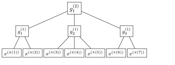
On its own terms, the paper claims that network sparsity is not the engine behind depth's ability to break the curse of dimensionality. Theorem 1 asserts that least squares estimation over the fully connected class $F(L_n, r_n)$, truncated at level $c_3 \log n$, attains $E\int|m_n(x)-m(x)|^2 P_X(dx) \le c_6 (\log n)^6 \max_{(p,K)\in P} n^{-2p/(2p+K)}$ whenever $m$ lies in the hierarchical composition class $H(l,P)$, with either $L_n\approx c_4\log n$ and $r_n\approx c_5\max n^{K/(2(2p+K))}$, or fixed width $r\approx c_8$ and $L_n\approx c_7\max n^{K/(2(2p+K))}\log n$. If true, practical dense architectures inherit the theoretical guarantees previously attached to carefully pruned sparse topologies.
Load-bearing premise
The load-bearing premise is that the true regression function is a finite-level hierarchical composition of smooth, Lipschitz inner functions with bounded derivatives, and that the level $l$ together with the smoothness/order set $P$ are known in advance; without that structure the dimension-free rate and the specified depth-width schedules have no foundation.
Editorial extensions
If this is right
- Sparse architectures are not needed for dimension-free rates; fully connected networks with the stated depth and width schedules are theoretically justified.
- The approximation error bound improves from $W^{-p/d}$ to $W^{-2p/d}$ in terms of total parameters for smooth functions on a cube.
- The same convergence rate is achievable in two regimes: constant width with polynomially growing depth, or logarithmically growing depth with polynomially growing width.
- Because the rate depends on the smoothness/order pairs in $P$ rather than on the ambient dimension $d$, hierarchical structure alone is enough to avoid the curse of dimensionality.
- Truncating the least squares estimator at level $c_3\log n$ is part of the construction and costs only logarithmic factors in the final bound.
Reading between the lines
- A testable practical extension is to replace the fixed constants $c_4,\dots,c_7$ with sample splitting or cross-validation over a grid of depths and widths; the rate should then hold adaptively without knowing $l$ and $P$, at the price of a further logarithmic factor.
- The approximation machinery is modular enough that the same proof strategy likely extends to other smoothness classes, such as Besov or mixed-smooth functions, provided the Taylor lemma is replaced by an appropriate local approximation statement.
- For applications, the fixed-width regime implies that very deep narrow networks are not merely an engineering choice but can be a theoretically optimal implementation; this suggests that pruning to constant-width subnetworks after training may preserve rates.
- The check-network and B-spline blending steps are tied to pointwise sup-norm control; an analogous argument in $L_2$ over the support of $X$ might require fewer shifted partitions and yield sharper constants.
Signed reviews
Editorial analysis
A structured set of objections, weighed in public.
Referee Report
Summary. The paper studies least-squares regression with fully connected ReLU networks of the form F(L,r) and proves that, for regression functions in a hierarchical composition class H(l,P) with finite level and known smoothness/order constraints, the L2 error is bounded by c (log n)^6 max_{(p,K) in P} n^{-2p/(2p+K)}. Two regimes are covered: logarithmic depth with growing width, and growing depth with fixed width. The authors develop new approximation theorems for (p,C)-smooth functions by fully connected ReLU networks, showing in particular that wide networks with W parameters achieve sup-norm approximation error of order W^{-2p/d}, and they propagate this approximation through the levels of the hierarchical composition. The proof combines the approximation results with standard empirical-process bounds and VC-dimension covering estimates.
Significance. The result is significant because it removes the sparsity constraint that was required in earlier dimension-free neural network regression theory (Schmidt-Hieber; Bauer-Kohler), demonstrating that a simple fully connected topology suffices for the same type of dimension-free rate when the regression function has modular structure. The approximation theorem also improves the parameter-count rate from O(epsilon^{-d/p}) to O(epsilon^{-d/(2p)}) for smooth functions, and the proposed architectures are explicitly implementable. The proof is detailed and essentially self-contained: the Taylor-polynomial and B-spline construction is developed from first principles, the composition induction is explicit, and the statistical part uses standard covering-number arguments. The main limitations, namely that the hierarchical level l and the constraint set P must be known and that the component functions need bounded derivatives and Lipschitz constants, are stated assumptions rather than hidden gaps.
minor comments (6)
- [Supplement B, Lemma 19] The inequality V_{T_beta F} <= V_F is stated without justification. Under the subgraph definition of VC dimension used in [6] it is correct, because subgraphs of T_beta f at thresholds t in (-beta,beta) coincide with subgraphs of f and thresholds outside this interval give empty or full sets; the authors should add this one-sentence justification or, if a different VC definition is intended, derive the bound from T_beta u = sigma(u+beta) - sigma(u-beta) - beta at the cost of one extra layer.
- [Supplement B, proofs of Lemmas 4, 5, 8] The cross-references in the supplement are incorrect: the proof of Lemma 4 cites Lemma 4 when it means the square-network Lemma 20, the proof of Lemma 8 cites Lemma 6 when it means the multiplier Lemma 4, and the proof of Lemma 5 cites Lemma 10 when it means the product-network Lemma 8.
- [Theorem 2 and Lemma 7] Several displayed depth formulas contain stray unmatched braces, for example the expression 'log_2(max{q, d} + 1})' in Theorem 2 and the analogous expression in Lemma 7; these should be cleaned up.
- [Theorem 1] The statement uses max over P and the proof chooses an argmin over P without assuming that P is finite; the statement should either assume P is finite or replace the max/argmin by the maximum over the finite set of pairs (p_g, K_g) that actually occur in the composition m.
- [Section 5, proof of Theorem 1] The phrase 'W.l.o.g. we assume supp(X) subset of [-a_n, a_n]^d' should say 'for n sufficiently large', since bounded support only guarantees containment in a fixed cube [-A,A]^d while a_n grows with n.
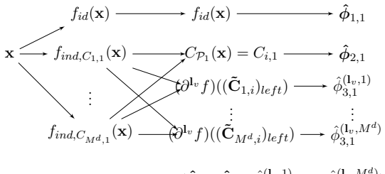
- [Theorems 1 and 3] The notation ||g||_{C^{q_g}(R^d)} is a type error: each g has input dimension K_g, so the norm should be taken on R^{K_g}; the same typo appears in the assumptions of Theorem 3.
Circularity Check
No circularity: the rate proof is self-contained and the hierarchical-composition rate is derived, not assumed.
full rationale
I walked the paper's derivation chain. Theorem 1 is obtained as a bias-variance decomposition: Lemma 18 bounds the stochastic error of the truncated least-squares estimator, Lemma 19 bounds the log-covering number of the fully connected ReLU class, and Theorem 3 supplies the approximation error for H(l,P). Theorem 3 itself is proved in Supplement A by composing the elementary approximation result Theorem 2, which is constructed from first principles using piecewise Taylor polynomials, ReLU indicator networks, multiplication networks, and 2^d shifted partitions. No step defines the target rate into existence: the rate max_{(p,K) in P} n^{-2p/(2p+K)} follows by choosing the approximation scales M_{j,i} = n^{1/(2(2p_j,i + K_j,i))} and balancing the resulting approximation term against the covering-number term, with the parameter bookkeeping checked explicitly in the proof of Theorem 1. The architecture choices L_n and r_n are prescribed functions of n and the known set P, not fitted to the data, so there is no fitted-input-called-prediction pattern. The self-citations that occur are not load-bearing in a circular sense: Lemma 18 is a standard empirical-process oracle inequality whose stated assumptions do not include the hierarchical composition class or the fully connected architecture; Lemmas 4, 5, 8 are marked as 'similar' to results in [33] but are proved in Supplement B; and the VC-dimension bound in Lemma 19 cites the independent result of Bartlett et al. [6]. Thus I cannot exhibit any equation or definition that reduces a claimed prediction to its own input, and the appropriate finding is no significant circularity.
Assumptions & free parameters
free parameters (1)
- Architecture constants c3, c4, c5, c7, c8 in Theorem 1
assumptions (6)
- standard math (p,C)-smoothness and Taylor approximation hold for the target and inner functions
- domain assumption The regression function m lies in the hierarchical composition class H(l,P)
- domain assumption Bounded support of X and E{exp(c1 Y^2)} < infinity
- domain assumption Each inner function g is Lipschitz continuous and has bounded derivatives up to its smoothness order
- standard math Existing empirical process and VC dimension bounds apply
- standard math Composition of fully connected ReLU networks with melted weights requires no extra layer
Cite this review
Pith. "Pith review of On the rate of convergence of fully connected very deep neural network regression estimates." pith.science (2026). https://pith.science/paper/ACTNW272
@misc{pith2026190811133,
  author       = {Pith},
  title        = {Pith review of: On the rate of convergence of fully connected very deep neural network regression estimates},
  year         = {2026},
  howpublished = {\url{https://pith.science/paper/ACTNW272}},
  note         = {Machine review of arXiv:1908.11133}
}
read the original abstract
Recent results in nonparametric regression show that deep learning, i.e., neural network estimates with many hidden layers, are able to circumvent the so-called curse of dimensionality in case that suitable restrictions on the structure of the regression function hold. One key feature of the neural networks used in these results is that their network architecture has a further constraint, namely the network sparsity. In this paper we show that we can get similar results also for least squares estimates based on simple fully connected neural networks with ReLU activation functions. Here either the number of neurons per hidden layer is fixed and the number of hidden layers tends to infinity suitably fast for sample size tending to infinity, or the number of hidden layers is bounded by some logarithmic factor in the sample size and the number of neurons per hidden layer tends to infinity suitably fast for sample size tending to infinity. The proof is based on new approximation results concerning deep neural networks.
Figures


Figures from the paper (4 more)



Forward citations
Cited by 3 Pith papers
-
Confidence Interval Construction and Conditional Variance Estimation with Dense ReLU Networks
Residual-based conditional variance estimation with dense ReLU networks achieves non-asymptotic rates under sub-Exponential noise, and a bootstrap interval for the conditional mean is proven to have coverage at least 1-alpha.
-
Dense ReLU Neural Networks for Temporal-spatial Model
Fully connected ReLU networks attain minimax-optimal nonparametric regression rates under temporal-spatial dependence with functional spatial noise, up to logarithmic factors.
-
Estimation of a function of low local dimensionality by deep neural networks
For regression functions that are locally low-dimensional, sparse neural network estimates achieve the rate n^{-2p/(2p+d*)}, with the exponent depending only on the local dimension d* and not the input dimension d.
Reference graph
Works this paper leans on
-
[1]
M. Anthony and P. L. Bartlett. Neural Network Learning: Theoretical Foundations . Cambridge University Press, New York, NY, USA, 1st edition, 2009
work page 2009
-
[2]
A. M. Bagirov, C. Clausen, and M. Kohler. Estimation of a re gression function by maxima of minima of linear functions. IEEE Trans. Inform. Theory , 55(2):833–845, 2009
work page 2009
-
[3]
A. Barron. Universal approximation bounds for superposi tions of a sigmoidal func- tion. IEEE Trans. Inform. Theory , 39(3):930–945, 1993
work page 1993
-
[4]
A. R. Barron. Complexity regularization with applicatio n to artificial neural net- works. Nonparametric Functional Estimation and Related Topics , pages 561–576, 1991
work page 1991
-
[5]
A. R. Barron. Approximation and estimation bounds for art ificial neural networks. Mach. Learn., 14(1):115–133, 1994
work page 1994
-
[6]
P. L. Bartlett, N. Harvey, C. Liaw, and A. Mehrabian. Nearl y-tight vc-dimension bounds for piecewise linear neural networks. J. Mach. Learn. Res. , 20:1–17, 2019
work page 2019
-
[7]
B. Bauer and M. Kohler. On deep learning as a remedy for the cu rse of dimensionality in nonparametric regression. Ann. Statist. , 47:2261–2285, 2019. 21
work page 2019
-
[8]
L. Devroye, L. Györfi, and G. Lugosi. A Probabilistic Theory of Pattern Recognition . Springer, 1996
work page 1996
Show all 63 references
-
[9]
L. P. Devroye and T. J. Wagner. Distribution-free consis tency results in nonparamet- ric discrimination and regression function estimation. Ann. Statist. , 8(2):231–239, 1980
1980
-
[10]
Eldan and O
R. Eldan and O. Shamir. The power of depth for feedforwar d neural networks. In V. Feldman, A. Rakhlin, and O. Shamir, editors, 29th Annual Conference on Learning Theory, volume 49 of Proc. Mach Learn. Res. (PMLR) , pages 907–940. PMLR, 2016
2016
-
[11]
U. Evci, F. Pedregosa, A. Gomez, and E. Elsen. The difficul ty of training sparse neural networks. CoRR, abs/1906.10732, 06 2019
1906 arXiv
-
[12]
J. H. Friedman and W. Stuetzle. Projection pursuit regr ession. J. Amer. Statist. Assoc., 76(376):817–823, 1981
1981
-
[13]
Grohs, D
P. Grohs, D. Perekrestenko, D. Elbrächter, and H. Bölcsk ei. Deep neural network approximation theory. IEEE Trans. Inform. Theory , 2019
2019
-
[14]
Györfi, M
L. Györfi, M. Kohler, A. Krzyżak, and H. Walk. A Distribution-Free Theory of Nonparametric Regression. Springer Series in Statistics. Springer, 2002
2002
-
[15]
Härdle, P
W. Härdle, P. Hall, and H. Ichimura. Optimal smoothing i n single-index models. Ann. Statist. , 21(1):157–178, 1993
1993
-
[16]
Härdle and T
W. Härdle and T. M. Stoker. Investigating smooth multip le regression by the method of average derivatives. J. Amer. Statist. Assoc. , 84(408):986–995, 1989
1989
-
[17]
S. Haykin. Neural Networks: A Comprehensive Foundation . Prentice Hall PTR, Upper Saddle River, NJ, USA, 2nd edition, 1998
1998
-
[18]
Hertz, R
J. Hertz, R. G. Palmer, and A. S. Krogh. Introduction to the Theory of Neural Computation. Perseus Publishing, 1st edition, 1991
1991
-
[19]
J. L. Horowitz and E. Mammen. Rate-optimal estimation f or a general class of nonparametric regression models with unknown link funct ions. Ann. Statist. , 35(6):2589–2619, 2007
2007
-
[20]
Imaizumi and K
M. Imaizumi and K. Fukumizu. Deep neural networks learn non-smooth functions effectively. Proc. Mach. Learn. Res. (PMLR) , 89:869–878, 2019
2019
-
[21]
M. Kohler. Optimal global rates of convergence for nois eless regression estimation problems with adaptively chosen design. J. Multivariate Anal. , 132:197 – 208, 2014
2014
-
[22]
Kohler and A
M. Kohler and A. Krzyżak. Adaptive regression estimati on with multilayer feedfor- ward neural networks. J. Nonparametr. Stat. , 17(8):891–913, 2005. 22
2005
-
[23]
Kohler and A
M. Kohler and A. Krzyżak. Nonparametric regression bas ed on hierarchical inter- action models. IEEE Trans. Inform. Theory , 63(3):1620–1630, 2017
2017
-
[24]
Kong and Y
E. Kong and Y. Xia. Variable selection for the single–in dex model. Biometrika, 94(1):217–229, 2007
2007
-
[25]
Z. Liu, M. Sun, T. Zhou, G. Huang, and T. Darrell. Rethink ing the value of network pruning. CoRR, abs/1810.05270, 2018
2018 arXiv
-
[26]
J. Lu, Z. Shen, H. Yang, and S. Zhang. Deep network approx imation for smooth functions. CoRR, arxiv:2001.03040, 2020
2001 arXiv
-
[27]
D. F. McCaffrey and A. R. Gallant. Convergence rates for s ingle hidden layer feedforward networks. Neural Networks, 7(1):147 – 158, 1994
1994
-
[28]
Mhaskar and T
H. Mhaskar and T. A. Poggio. Deep vs. shallow networks : A n approximation theory perspective. Anal. Appl. (Singap.) , 14, 2016
2016
-
[29]
Ohn and Y
I. Ohn and Y. Kim. Smooth function approximation by deep neural networks with general activation function. Entropy, 21(7):627–647, 2019
2019
-
[30]
Oono and T
K. Oono and T. Suzuki. Approximation and nonparametric estimation of resnet-type cpnvolutional neural networks. In K. Chaudhuri and R. Salak hutdinov, editors, Pro- ceedings of the 36th International Conference on Machine Learning, volume 97, pages 4922–4931, Long Beach, Calif...
2019
-
[31]
B. D. Ripley and N. L. Hjort. Pattern Recognition and Neural Networks . Cambridge University Press, New York, NY, USA, 1st edition, 1995
1995
-
[32]
Schmidhuber
J. Schmidhuber. Deep learning in neural networks: An ov erview. Neural Networks, 61:85–117, 2015
2015
-
[33]
Schmidt-Hieber
J. Schmidt-Hieber. Nonparametric regression using de ep neural networks with relu activation function. Ann. Statist. , 48(4):1875–1897, 2020
2020
-
[34]
C. J. Stone. Optimal global rates of convergence for non parametric regression. Ann. Statist., 10(4):1040–1053, 1982
1982
-
[35]
C. J. Stone. Additive regression and other nonparametr ic models. Ann. Statist. , 13(2):689–705, 1985
1985
-
[36]
C. J. Stone. The use of polynomial splines and their tens or products in multivariate function estimation. Ann. Statist. , 22(1):118–171, 1994
1994
-
[37]
T. Suzuki. Adaptivity of deep ReLU network for learning in Besov and mixed smooth Besov spaces: optimal rate and curse of dimensionality. International conference on learning representations, 2019
2019
-
[38]
Yarotsky
D. Yarotsky. Optimal approximation of continuous func tions by very deep relu networks. COLT, 75:639–649, 2018. 23
2018
-
[39]
Yarotsky and A
D. Yarotsky and A. Zhevnerchuk. The phase diagram of app roximation rates for deep neural networks. CoRR, abs/1906.09477, 2019
1906 arXiv
-
[40]
bottom left
Y. Yu and D. Ruppert. Penalized spline estimation for pa rtially linear single-index models. J. Amer. Statist. Assoc. , 97(460):1042–1054, 2002. A. APPENDIX: NETWORK APPROXIMATION OF SMOOTH FUNCTIONS A.1. Proof of Theorem 2 In this section we prove Theorem 2. The main idea is ...
2002
-
[41]
Compute Tf,q, (CP2 (x))lef t(x) by using recursively defined functions
-
[42]
The resulting network is a good approximation for f (x) in case that x ∈ ⋃ k∈{1,...,M 2d} (Ck, 2)0 1/M 2p+2
Approximate the recursive functions by neural networks. The resulting network is a good approximation for f (x) in case that x ∈ ⋃ k∈{1,...,M 2d} (Ck, 2)0 1/M 2p+2. 25
-
[43]
Construct a neural network to approximate wP2(x) · f (x), where wP2(x) = d∏ j=1 ( 1 − M 2 a · ⏐ ⏐ ⏐(CP2 (x))(j) lef t + a M 2 − x(j) ⏐ ⏐ ⏐ ) + is a linear tensorproduct B-spline which takes its maximum va lue at the center of CP2(x), which is nonzero in the inner part of CP2(x...
-
[44]
Apply those networks to 2d slightly shifted partitions of P2 to approximate f (x) in supremum norm. A.1.4. Key step 1: A recursive definition of Tf,q, (CP2 (x))lef t(x) The following recursive definition of the piecewise Taylor p olynomial will later help us to define a neural ne...
-
[45]
is contained in the interval where ( 19) holds. By choosing BM,p = ⌈log4 ( M 2p) ⌉ we get ⏐ ⏐ ⏐fnet, P2(x) − Tf,q, (CP2 (x))lef t(x) ⏐ ⏐ ⏐ = ⏐ ⏐ ⏐ˆφ1, 3 − φ1, 3 ⏐ ⏐ ⏐ ≤ c36 · ( max { 2a, ‖f ‖Cq([−a,a ]d) })4(q+1) · 1 M 2p , where we have used ¯r(p) ≤ 1. This together with Lemm...
-
[46]
a value not equal to zero, this leads to ⏐ ⏐ ⏐ˆφ(l) 3, 2 ⏐ ⏐ ⏐ ≤ ‖f ‖Cq([−a,a ]d) and ⏐ ⏐ ⏐ˆφ(s) 2, 2 ⏐ ⏐ ⏐ ≤ a, (s ∈ {1, . . . , d}). We conclude |fnet, P2(x)| ≤ ⏐ ⏐ ⏐fp ( z, y1, . . . , y(d+q d ) ) − p ( z, y1, . . . , y(d+q d ) )⏐ ⏐ ⏐ + ⏐ ⏐ ⏐p ( z, y1, . . . , y(d+q d ) )⏐ ...
-
[47]
Thus we say that this network checks the position of our input x
and 0 if x is contained in ⋃ k∈{1,...,M 2d} (Ck, 2)0 2/M 2p+2. Thus we say that this network checks the position of our input x. A straightforward way to approximate 1⋃ k∈{ 1,...,M 2d } Ck, 2\(Ck, 2)0 1/M 2p+2 (x) = 1 − ∑ k∈{1,...,M 2d} 1(Ck, 2)0 1/M 2p+2 (x) by a neural netwo...
-
[48]
Summarizing this we can conclude that 1 − f2(x) − f 2 id( ˆf1(x)) = ∑ j∈{1,...,M d} 1( ˜Cj,i )0 1/M 2p+2 (x) − f 2 id( ˆf1(x)) ≤ 0 − 0 = 0
holds we further have ˆf2(x) = f2(x) as shown in the second case. Summarizing this we can conclude that 1 − f2(x) − f 2 id( ˆf1(x)) = ∑ j∈{1,...,M d} 1( ˜Cj,i )0 1/M 2p+2 (x) − f 2 id( ˆf1(x)) ≤ 0 − 0 = 0 . This implies fcheck, P2(x) = 1 − 0 = 1 = 1⋃ k∈{ 1,...,M 2d} Ck, 2\(Ck,...
-
[49]
holds. Together with wP2(x) ≤ 1 a · M 2p and the triangle inequality it follows ⏐ ⏐ ⏐fmult ( fwP2 (x), fnet, P2,true (x) ) − wP2(x) · f (x) ⏐ ⏐ ⏐ ≤ ⏐ ⏐ ⏐fmult ( fwP2 (x), fnet, P2,true (x) ) − fwP2 (x)fnet, P2,true (x) ⏐ ⏐ ⏐ + ⏐ ⏐ ⏐fwP2 (x) · fnet, P2,true (x) − wP2(x) · fnet,...
-
[50]
Compute ˆTf,q, (CP2 (x))lef t(x) by recursively defined functions
-
[51]
The resulting network is a good approximation for f (x) in case that x ∈ ⋃ k∈{1,...,M 2d} (Ck, 2)0 1/M 2p+2
Approximate the recursive functions by neural networks. The resulting network is a good approximation for f (x) in case that x ∈ ⋃ k∈{1,...,M 2d} (Ck, 2)0 1/M 2p+2
-
[52]
Approximate the function wP2(x) · f (x) by deep neural networks
-
[53]
Apply those networks to 2d slightly shifted partitions of P2 to approximate f (x) in supremum norm. A.1.9. Key step 1: A recursive definition of ˆTf,q, (CP2 (x))lef t(x) As in the proof of Theorem 2 a) we will use that we can compute ˆTf,q, (CP2 (x))lef t(x) recursively. To do ...
-
[54]
and we have A(j) = ˜Cj,i . Furthermore we can conclude that φ(l) 3,M d+j = (∂l ˆf )(( ˜Cj+1,i )lef t), where we have used that φ(l) 4,M d+j−1 = M d−j∑ k=1 (b(l) k+j−1,i + ⌈ed⌉ + 2) · (4 + 2⌈ed⌉)−k and ⌊(4 + 2 · ⌈ed⌉) · φ(M d+j−1) 4, l ⌋ − ⌈ed⌉ − 2 = b(l) j,i . This leads to φ ...
-
[55]
We get ⏐ ⏐ ⏐fnet,deep, P2(x) − ˆTf,q, (CP2 (x))lef t(x) ⏐ ⏐ ⏐ = ⏐ ⏐ ⏐ˆφ1, 2M d+1 − φ1, 2M d+1 ⏐ ⏐ ⏐ 66 ≤ c36 · (6 + 2⌈ed⌉)4(q+1) · ( 2 · max { a, ‖f ‖Cq([−a,a ]d) })4(q+1) · 1 M 2p
is contained in the interval, where ( 38) holds. We get ⏐ ⏐ ⏐fnet,deep, P2(x) − ˆTf,q, (CP2 (x))lef t(x) ⏐ ⏐ ⏐ = ⏐ ⏐ ⏐ˆφ1, 2M d+1 − φ1, 2M d+1 ⏐ ⏐ ⏐ 66 ≤ c36 · (6 + 2⌈ed⌉)4(q+1) · ( 2 · max { a, ‖f ‖Cq([−a,a ]d) })4(q+1) · 1 M 2p . This together with Lemma 1 and (36) shows the...
-
[56]
and ( 40) a value not equal to zero, this leads to ⏐ ⏐ ⏐ˆφ(k) 5, 2M d ⏐ ⏐ ⏐ ≤ a (k ∈ {1, . . . , d}) and ⏐ ⏐ ⏐ˆφ(l) 6, 2M d ⏐ ⏐ ⏐ ≤ ‖f ‖Cq([−a,a ]d) · e(M d−1)·2ad/M 2 + (4 + 2 · ⌈ed⌉) · M d−2∑ k=0 ek·2ad/M 2 ≤ ‖f ‖Cq([−a,a ]d) · e(M d−1) + (4 + 2 · ⌈ed⌉) · (M d − 1) · e(M d−2...
-
[57]
, y(d+q d ) ) − p ( z, y1,
holds, we can bound the value of fnet,deep, P2(x) by |fnet,deep, P2(x)| ≤ ⏐ ⏐ ⏐fp ( z, y1, . . . , y(d+q d ) ) − p ( z, y1, . . . , y(d+q d ) )⏐ ⏐ ⏐ + ⏐ ⏐ ⏐p ( z, y1, . . . , y(d+q d ) )⏐ ⏐ ⏐ ≤ 1 + ⏐ ⏐ ⏐ ⏐ ⏐ ∑ l∈Nd 0 ‖l‖1≤q 1 l! · ( ‖f ‖Cq([−a,a ]d) · e(M d−1) + (4 + 2 · ⌈ed⌉)...
-
[58]
we can conclude that ⏐ ⏐ ⏐ˆh(1) j (x) − h(1) j (x) ⏐ ⏐ ⏐ ≤ c50 · 1 · (Kmax · CLip)1−1 · a4·(pmax+1) · max j,i M −2p(i) j j,i for j ∈ { 1, . . . , ˜N1}. Thus we have shown that (
-
[59]
Assume now that (44) holds for some i − 1 and every j ∈ {1,
holds for i = 1 . Assume now that (44) holds for some i − 1 and every j ∈ {1, . . . , ˜Ni−1}. Then ⏐ ⏐ ⏐ˆh(i−1) j (x) ⏐ ⏐ ⏐ ≤ ⏐ ⏐ ⏐ˆh(i−1) j (x) − h(i−1) j (x) ⏐ ⏐ ⏐+ gmax ≤ 2 · gmax follows directly by the induction hypothesis. Using (
-
[60]
,ˆh(i−1) ∑ j t=1 K (i) t ) −g(i) j ( ˆh(i−1) ∑ j− 1 t=1 K (i) t +1 ,
and the Lipschitz continuity of g(i) j we can conclude that ⏐ ⏐ ⏐ˆh(i) j (x) − h(i) j (x) ⏐ ⏐ ⏐ ≤ ⏐ ⏐ ⏐ ⏐fnet,wide,g (i) j ( ˆh(i−1) ∑ j− 1 t=1 K (i) t +1 , . . . ,ˆh(i−1) ∑ j t=1 K (i) t ) −g(i) j ( ˆh(i−1) ∑ j− 1 t=1 K (i) t +1 , . . . ,ˆh(i−1) ∑ j t=1 K (i) t )⏐ ⏐ ⏐ ⏐ + ⏐ ⏐...
-
[61]
, ˜N1}) is contained in the interval, where inequality ( 45) holds
holds for i = 1 and that the output of each hi(x) ( i ∈ {1, . . . , ˜N1}) is contained in the interval, where inequality ( 45) holds. Assume now that (46) holds for some i − 1 and every j ∈ {1, . . . , ˜Ni−1}. Then ⏐ ⏐ ⏐ ⏐ˆhN (i− 1) j (x) ⏐ ⏐ ⏐ ⏐ ≤ ⏐ ⏐ ⏐ ⏐ˆhN (i− 1) j (x) − hN...
-
[62]
, d} and any z1, z2 ∈ [−(4l − 1) · al, (4l − 1) · al] |fmult(z1, z2)| ≤ | z1 · z2| + |fmult(z1, z2) − z1 · z2| ≤ (4l − 1)2a2l + 1 ≤ (42l − 1) · a2l
and R ≥ log4 ( 2 · 42·d · a2·d) we get for any l ∈ { 1, . . . , d} and any z1, z2 ∈ [−(4l − 1) · al, (4l − 1) · al] |fmult(z1, z2)| ≤ | z1 · z2| + |fmult(z1, z2) − z1 · z2| ≤ (4l − 1)2a2l + 1 ≤ (42l − 1) · a2l. From this we get successively that all outputs of layer l ∈ {1, . ...
-
[63]
and the fact that all outputs of layer l ∈ {1, . . . , q − 1} are contained in the interval [−42l a2l , 42l a2l ]) we get for x ∈ [−a, a]d |fmult,d (x) − d∏ i=1 x(i)| ≤ ∆ q ≤ 2 · (4d · ad)2 · 4−R · 41+2+···+2q− 1 · a1+2+···+2q− 1 · ( 1 + 2 + · · · + 2q−1) ≤ (4d · ad)2 · 4−R · ...
Reviewed August 14, 2026 · model on record in the stance chip above.
Discussion (0). Continue with ORCID to comment.