REVIEW 3 major objections 5 minor 113 references
Classifying single-qubit noise using machine learning
T0 review · 3 major / 5 minor · reviewed 2026-08-14 · deepseek-v4-flash
Pith's one-line read This paper reports that machine-learning classifiers can distinguish coherent from stochastic single-qubit noise using gate set tomography data, and that the two classes become linearly separable after feature engineering.
desk verdict A careful ML-for-QCVV proof of principle whose central claim is undercut by a mean-generator asymmetry between the two simulated noise classes. read the letter →
The pith
A machine-rendered reading of the paper's core claim, the machinery that carries it, and where it could break.
The reading
What carries the argument
The central object is the decision surface learned by a supervised classifier, viewed geometrically as a surface that separates gate set tomography feature vectors labeled “coherent” from those labeled “stochastic”. The argument is carried by two pieces: a linear-programming test for linear separability that can certify, via a theorem of alternatives, when no separating hyperplane exists; and the feature maps $\varphi_{\mathrm{SQ}}$ and $\varphi_{\mathrm{PP}}$, which append $f_j^2$ or $f_j f_k$ terms to the raw outcome-frequency vector and thereby unroll the curved “radio dish” geometry of the shallowest GST data so that a hyperplane can separate the classes. The geometric margin of the learned hyperplane is what connects training accuracy to robustness under finite-sample noise.
What would settle it
Regenerate both training ensembles with matched first- and second-order error statistics -- for example, zero-mean Hamiltonian perturbations for coherent noise and zero-mean Lindblad jump coefficients for stochastic noise, with equal variances -- then retrain the same classifiers. If accuracy falls to chance, the original separation was driven by the average-error-size confound rather than by coherence.
Extended reading notes
Core claim
The paper's central claim is that a supervised classifier can learn to distinguish coherent from stochastic single-qubit noise directly from gate set tomography (GST) data, without constructing a statistical noise model. For GST experiment designs with circuit depth index $L>1$, the paper finds that the collections of simulated GST frequencies are linearly separable: a hyperplane can separate feature vectors generated by coherent noise from those generated by stochastic noise with near-perfect accuracy once hyperparameters are tuned. For the shallowest design ($L=1$), the raw data are not linearly separable, but the paper proves that they become linearly separable after adding polynomial features -- the squares of individual outcome frequencies or all pairwise products -- and that linear classifiers then match intrinsically nonlinear ones. The paper also demonstrates that a maximum-margin linear SVM trained on noiseless engineered features handles finite-sampling noise reliably once the statistical fluctuations are below the hyperplane's geometric margin. The intended lesson is that off-the-shelf machine learning can automatically produce a working quantum-characterization data-processing map for this simplified binary property.
Load-bearing premise
The load-bearing premise is that the simulated experiments isolate coherence as the thing that differs between the two classes; in fact the stochastic-noise ensemble has a nonzero average error that grows with the noise-strength parameter while the coherent-noise ensemble has zero-mean error, so the classifier may be detecting error magnitude rather than coherence itself.
Editorial extensions
If this is right
- A user could classify the noise on a qubit as coherent or stochastic by running standard GST circuits and applying a trained linear classifier, with no need to fit a full gate set or choose a noise model.
- Increasing the GST circuit-depth index improves separability: for $L>1$, raw outcome frequencies are linearly separable, so a hyperplane classifier reaches high accuracy after hyperparameter tuning.
- Feature engineering such as $\varphi_{\mathrm{SQ}}$ or $\varphi_{\mathrm{PP}}$ makes even the shallowest GST design linearly separable, showing that the information distinguishing the two noise types is present in short circuits but requires nonlinear feature maps to expose.
- A maximum-margin SVM is a practical choice for this task because its accuracy degrades gracefully as finite-sample noise is added, staying essentially perfect once $1/\sqrt{N_{\mathrm{samples}}}$ falls below the margin.
- The same rubric and training-data approach could be reused for other single-qubit properties, since only the property labels and performance measure would need to change.
Reading between the lines
- The simulated ensembles are not matched in their first-order statistics: stochastic noise has a nonzero average error generator proportional to the noise strength, while coherent noise has zero-mean Hamiltonian perturbations. The reported classifiers may therefore be solving a magnitude-detection problem in disguise, and a test with matched error moments would separate ‘coherence’ from ‘size of er
- The “radio dish” structure seen in the low-dimensional embeddings suggests the coherence label is recoverable from distance-like quantities in a Choi-state picture, where pure states envelop mixed states; if so, a single hand-designed invariant such as the purity of the estimated process would probably give the same separation, making the engineered polynomial features a data-driven stand-in for t
- A natural extension, implicit in the paper's own discussion, is a regression version that estimates a continuous coherence measure (such as unitarity) from the same GST data; the high accuracies reported for the binary problem suggest that regression target should also be learnable.
- If this recipe generalizes beyond one qubit, quantum device diagnostics could be built as libraries of trained classifiers attached to fixed experiment designs, with experts contributing labels rather than statistical models; the dominant obstacle would be generating representative training data as processors grow.
Signed reviews
Editorial analysis
A structured set of objections, weighed in public.
Referee Report
Summary. This paper proposes a rubric for developing 'machine-learned' QCVV protocols, in which a supervised classifier replaces the statistical model and estimator of a conventional QCVV pipeline, and applies that rubric to the binary task of deciding whether single-qubit gate noise is coherent or stochastic. Training data are synthetic GST data sets produced by pyGSTi simulations of two noise ensembles: Gaussian unitary (coherent) perturbations and random-basis Lindblad (stochastic) decay. For each GST experiment design index L, the authors test linear separability with a linear program whose dual certifies inseparability, evaluate five classifiers under default and tuned hyperparameters, examine the low-dimensional structure of the L=1 data via PCA and MDS, introduce two quadratic feature maps that restore linear separability for L=1, and show that an SVM's margin predicts robustness to finite-sample noise. The main empirical claims are that GST data sets are linearly separable for L>1, that the L=1 data have a 'radio dish' geometry, and that feature engineering lets linear classifiers match or approach nonlinear ones.
Significance. As a proof of principle for using ML to learn QCVV data-processing maps, the paper is executed with unusual care: linear separability is certified by an LP with a dual witness, hyperparameters are tuned by explicit grid search, generalization is checked by repeated cross-validation and held-out 'hero tests', and the simulations use the standard pyGSTi toolchain. The rubric in Section II is a genuinely useful contribution that could structure future work in this area. However, the central demonstration is undermined by a mismatch between the two generative noise ensembles: the stochastic ensemble has a nonzero first-order generator mean while the coherent ensemble does not, so the learned decision surfaces may be separating on a first-order error-magnitude signal rather than on coherence. This is a fixable but load-bearing issue; with a matched-strength or per-η analysis, the paper could support its claims, but as written the claim that ML can learn to distinguish coherent from stochastic noise is not established.
major comments (3)
- [Appendix A, Eqs. (A4)-(A11); Section III.1] The two simulated noise classes differ not only in coherence but in their first-order average generator. Coherent errors are drawn from a zero-mean Gaussian Hamiltonian (Eq. (A4), with ⟨He⟩=0 in Eq. (A9)), while the stochastic rates are drawn from a folded normal (Eq. (A8)) whose mean is nonzero: Eq. (A11) gives ⟨h_jk⟩ ∝ η > 0. Since η spans 10^-4 to 0.5 with equal sample counts per class, a linear classifier can attain high pooled accuracy by thresholding on the systematic O(η) dissipative shift rather than on coherence, and the confound survives at fixed η because the mean shift itself is proportional to η. This contradicts the paper's own definition in Section III.1 that stochastic errors are zero-mean fluctuations; the nonzero mean is computed in Eq. (A11) but never analyzed in the results. The central claim that the learned classifiers distinguish coherent from stochastic noise therefore requires a matched-error-strength control, per-η accuracy reporting, or an explicit analysis showing that the decision surface does not rely on the first-order generator.
- [Table III; Section IV A 1] The paper's restricted-η separability checks do not resolve the confound. Table III reports that fixed-η subsets of C1 are linearly separable, but this is exactly what a separator acting on the O(η) mean displacement of the stochastic ensemble would produce; separability at fixed η does not demonstrate separation on the basis of coherence. Similarly, the undersampling check in Table IV compares train and test accuracy pooled over all η values, so the ~0.97 test accuracy is also consistent with a mean-threshold explanation. Because no per-η accuracies, confusion matrices, or feature-ablation results are reported anywhere in Section IV, the proxy hypothesis is not ruled out by the present data.
- [Section IV E, Figure 9] The finite-sample robustness demonstration is internal to the confounded generative model: the SVM is trained and evaluated on the same folded-normal stochastic ensemble, so the computed margin and the accuracy-vs-noise curves certify robustness of a mean-shift separator rather than of a coherence classifier. The claim that the φSQ and φPP feature maps do not increase finite-sample sensitivity is likewise evaluated only on this ensemble. This section should be re-run, or at minimum reinterpreted, once the ensemble-matching issue is addressed.
minor comments (5)
- [Section III 4 b] In the RBF SVM paragraph, 'in the original feautre space' should read 'feature space'.
- [References, [59]] Reference [59] is broken: the sentence 'We use “◦.' is incomplete and should be finished or removed.
- [Figure 6] The caption does not state what the points in the swarmplot represent (presumably per-fold accuracies across the K=20 splits); this should be clarified, and error bars or a box plot would improve readability.
- [Section IV B] The 'radio dish' interpretation is presented as strongly supported by the Choi-Jamiolkowski analogy, but the argument is explicitly heuristic (the text concedes 'the exact structure may not be comparable'); the qualitative claim should be labeled as such or backed by a quantitative test.
- [Section IV A 1 and Appendix C] The statement that 'we do not use the extra 20900 feature vectors' appears in both Section IV A 1 and Appendix C; the hero-test procedure should be described once and referenced thereafter.
Circularity Check
No significant circularity: classifier training and evaluation use standard supervised learning on held-out simulated data.
full rationale
The paper's central claim is that supervised classifiers can learn to separate GST feature vectors generated by coherent versus stochastic single-qubit noise. The derivation chain is an empirical ML pipeline: (i) the two noise classes are defined by explicit generator models (Appendix A, Eqs. A2-A8); (ii) GST circuits provide the feature map (Eq. 7); (iii) classifiers are trained on one set of simulated data and evaluated on held-out data using cross-validation and separate hero tests; and (iv) linear separability is certified by an LP feasibility/duality argument (Appendix B). No fitted parameter is renamed as a prediction, no equation defining the target is reused as the learned map, and no load-bearing premise is justified solely by a self-citation. The GST and pyGSTi citations are tooling and background, not arguments that force the result. The paper's main vulnerability is a potential confound: the stochastic ensemble has a nonzero mean generator (Eq. A11) even though Section III.1 defines stochastic fluctuations as having zero expected value, so the classifier may partly learn a first-order error-magnitude signal rather than coherence. That is a correctness or validity concern, not circularity, because the learned decision surface is not equal to its training input by construction. Accordingly, the circularity score is 0.
Assumptions & free parameters
free parameters (2)
- Noise strength η grid =
19 values: {1,2.15,4.64}×10^{-4}, {1,2.15,4.64}×10^{-3}, {1,2.15,4.64}×10^{-2}…
- Algorithm hyperparameters (LDA τ, QDA s, SVM C and γ, perceptron Nepochs) =
Grid values listed in Table II
assumptions (5)
- domain assumption Noise is Markovian and time-independent; each gate is replaced by the same CPTP map throughout a circuit.
- ad hoc to paper Purely coherent errors are generated by a zero-mean Gaussian unitary Hamiltonian perturbation, while purely stochastic errors are generated by Lindblad decay rates drawn from a folded normal with a random basis.
- domain assumption GST circuits are sufficient to infer any Markovian property, including coherent versus stochastic noise.
- standard math LP duality (theorem of alternatives) correctly certifies linear separability or provides a witness of inseparability.
- domain assumption Cross-validation on the simulated distribution estimates generalization within that distribution.
Cite this review
Pith. "Pith review of Classifying single-qubit noise using machine learning." pith.science (2026). https://pith.science/paper/GI4MG67O
@misc{pith2026190811762,
  author       = {Pith},
  title        = {Pith review of: Classifying single-qubit noise using machine learning},
  year         = {2026},
  howpublished = {\url{https://pith.science/paper/GI4MG67O}},
  note         = {Machine review of arXiv:1908.11762}
}
read the original abstract
Quantum characterization, validation, and verification (QCVV) techniques are used to probe, characterize, diagnose, and detect errors in quantum information processors (QIPs). An important component of any QCVV protocol is a mapping from experimental data to an estimate of a property of a QIP. Machine learning (ML) algorithms can help automate the development of QCVV protocols, creating such maps by learning them from training data. We identify the critical components of "machine-learned" QCVV techniques, and present a rubric for developing them. To demonstrate this approach, we focus on the problem of determining whether noise affecting a single qubit is coherent or stochastic (incoherent) using the data sets originally proposed for gate set tomography. We leverage known ML algorithms to train a classifier distinguishing these two kinds of noise. The accuracy of the classifier depends on how well it can approximate the "natural" geometry of the training data. We find GST data sets generated by a noisy qubit can reliably be separated by linear surfaces, although feature engineering can be necessary. We also show the classifier learned by a support vector machine (SVM) is robust under finite-sample noise.
Figures


Figures from the paper (7 more)


Reference graph
Works this paper leans on
-
[1]
Are the gate errors coherent or stochastic?
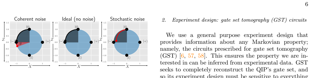
Property P: “Are the gate errors coherent or stochastic?” The single-qubit QIP we consider will be assumed to have five operations: initialization of some fiducial state ρ0, three logic gates corresponding to idling and π/2 ro- tations around the X and Y axes of the Bloch sphere (GI,GX, and GY , respectively), and a terminating mea- surement, E. The collect...
-
[2]
coherent vs. stochastic
Experiment design: gate set tomography (GST) circuits We use a general purpose experiment design that provides information about any Markovian property; namely, the circuits prescribed for gate set tomography (GST) [6, 57, 58]. This ensures the property we are in- terested in can be inferred from experimental data. GST seeks to completely reconstruct the ...
-
[3]
The em- bedding is described by a feature map, φ, mapping each QCVV data setD to a feature vector f (i.e.,φ :D→ f∈ F)
A feature map φ for embedding data into a feature space Making QCVV data amenable to analysis by ML al- gorithms requires embedding it into a feature space,F, which is typically isomorphic to Rn for some n. The em- bedding is described by a feature map, φ, mapping each QCVV data setD to a feature vector f (i.e.,φ :D→ f∈ F). If ML algorithms do not perform...
-
[4]
For example, properties that are categorical would re- quire classification algorithms, whereas properties that are continuous would require regression algorithms
A data processing pipeline, centered around an ML algorithmA The choice of algorithmA depends strongly onP and the kind of QCVV data the algorithm will have access to. For example, properties that are categorical would re- quire classification algorithms, whereas properties that are continuous would require regression algorithms. In addition, if the traini...
-
[5]
It measures the quality of fθ’s predictions
A performance measure P used to evaluate predictions Some measure of performance is necessary to evaluate whether a given map fθ is a good one. It measures the quality of fθ’s predictions. Typically, the performance measure is defined in terms of a loss function to quantify the penalty for an incorrect prediction. For binary or discrete classification, the ...
-
[6]
In simple cases the hyperparameters can be specified a priori
A specification of (or search protocol over) the algorithm’s hyperparameters Hyperparameters are user-controllable parameters that affect the algorithm’s behavior, and the algorithm’s performance depends on their values. In simple cases the hyperparameters can be specified a priori . In other cases, a procedure for varying the hyperparameters to find good val...
-
[7]
Estimate the coherence of noise
Labeled training data from which the algorithm can learn ML algorithms learn using training data. Conse- quently, a machine-learned QCVV technique requires a collection of training data C that the ML algorithm can learn from. In supervised learning, each data set Dj in the collection carries with it a label defined by an instance of the property of interes...
-
[8]
L =l GST feature vector
Feature space F: the unit hypercube A GST data set is usually presented as a list of count statistics, one for each circuit. But ML algorithms rep- 7 0 50 100 150 200 250 GST experiment design index L 0 500 1000 1500 2000 2500Feature space dimension d FIG. 4. Feature space dimensiond grows with the GST experiment design index L. We use a simple feature ma...
2000
Show all 113 references
-
[9]
Given a collection of feature vectors C = {(fj,yj)}N j=1, with yj ∈ {±1} indicating which class the feature vector fj∈F belongs to, learn a classifier c :F→{± 1}
Algorithm A: supervised binary classifiers We use supervised classifiers because synthetic train- ing data can be easily generated. The general task of supervised learning (for binary classification) is: “Given a collection of feature vectors C = {(fj,yj)}N j=1, with yj ∈ {±1} in...
-
[10]
0/1 loss
Performance measure P To search over its hypothesis class, an ML algorithm needs a measure of how good any hypothesis in the class is. Here, we use a simple performance measure for a given hypothesis: A = { 1 if c(fj) =yj 0 otherwise , (18) for which the average accuracy equal...
-
[11]
For each algorithm, we performed hyperparameter tuning using brute-force grid search over the values listed in Table II; see Appendix C for details
Hyperparameter specification All of the algorithms discussed in Section III 4 b have hyperparameters that affect their behavior. For each algorithm, we performed hyperparameter tuning using brute-force grid search over the values listed in Table II; see Appendix C for details
-
[12]
stochas- tic
Data collection C We generated a large collection of labeled training data – simulated GST datasets for many realizations of purely stochastic and coherent noise – which we use for train- ing and cross-validation. To produce this data, we nu- merically simulated GST data sets ...
-
[13]
linear GST
Testing whether linear classification is feasible Three of the classification algorithms presented in Sec- tion III 4 learn a linear decision surface. If CL is not linearly separable, then those algorithms cannot perform well. So for eachL, we began our analysis by determining w...
-
[14]
uninformative
Classification accuracy depends on L, and hyperparameter tuning is necessary WhenCL is linearly separable, a linear classifier could in principle successfully learn a separating hyperplane. Whether such an algorithm succeeds in practice depends very much on its hyperparameters. ...
-
[15]
Hero test
In the conclusions (Section V) we discuss how ML could also be used to construct experiment designs. 19 Algorithm φ Hyperparameter value Mean accuracy (K = 20 cross- validation) “Hero test” accuracy LDA PP 10−1 0.87 0.87 LDA SQ 10−5 0.86 0.867 Linear SVM PP 75 0.991 0.97 Linea...
-
[16]
Preskill, Quantum 2, 79 (2018), arXiv:1801.00862
J. Preskill, Quantum 2, 79 (2018), arXiv:1801.00862
2018 arXiv
-
[17]
A Preview of Bristlecone, Google’s New Quan- tum Processor,
J. Kelly, “A Preview of Bristlecone, Google’s New Quan- tum Processor,” (2018)
2018
-
[18]
IBM Announces Advances to IBM Quantum Sys- tems & Ecosystem,
C. Vu, “IBM Announces Advances to IBM Quantum Sys- tems & Ecosystem,” (2017)
2017
-
[19]
Wright, K
K. Wright, K. M. Beck, S. Debnath, J. M. Amini, Y. Nam, N. Grzesiak, J. S. Chen, N. C. Pisenti, M. Chmielewski, C. Collins, K. M. Hudek, J. Mizrahi, J. D. Wong-Campos, S. Allen, J. Apisdorf, P. Solomon, M. Williams, A. M. Ducore, A. Blinov, S. M. Kreike- meier, V. Chaplin, M. ...
1903 arXiv
-
[20]
Unsupervised Machine Learning on Rigetti 19Q with Forest 1.2,
W. Zeng, “Unsupervised Machine Learning on Rigetti 19Q with Forest 1.2,” (2017)
2017
-
[21]
Blume-Kohout, J
R. Blume-Kohout, J. K. Gamble, E. Nielsen, J. Mizrahi, J. D. Sterk, and P. Maunz, arXiv:1310.4492
-
[22]
Magesan, J
E. Magesan, J. M. Gambetta, and J. Emerson, Physical Review Letters 85, 042311 (2012)
2012
-
[23]
Magesan, J
E. Magesan, J. M. Gambetta, and J. Emerson, Physical Review Letters 106, 180504 (2011), arXiv:1009.3639
2011 arXiv
-
[24]
A. W. Cross, L. S. Bishop, S. Sheldon, P. D. Nation, and J. M. Gambetta, arXiv:1811.12926
- [25]
-
[26]
A. L. Samuel, IBM Journal of Research and Development 3, 210 (1959)
1959
-
[27]
Hastie, R
T. Hastie, R. Tibshirani, and J. Friedman, The Elements of Statistical Learning, 2nd ed. (Springer, 2016)
2016
-
[28]
Goodfellow, Y
I. Goodfellow, Y. Bengio, A. Courville, and F. Bach, Deep Learning (MIT Press, 2016) p. 775
2016
-
[29]
James, D
G. James, D. Witten, T. Hastie, and R. Tibshirani, An Introduction to Statistical Learning: with Applications in R, 7th ed. (Springer, 2017)
2017
- [30]
-
[31]
For example, the model in randomized benchmarking predicts certain averages, rather than individual circuit probabilities
-
[32]
Wasserman, All of Statistics: A Concise Course in Statistical Inference (Springer New York, 2004)
L. Wasserman, All of Statistics: A Concise Course in Statistical Inference (Springer New York, 2004)
2004
-
[33]
G. E. P. Box, in Workshop on Robustness in Statistics , edited by R. L. Launer and G. N. Wilkinson (Academic Press, Research Triangle Park, North Carolina, USA,
-
[34]
Some ML algorithms are in fact universal function ap- proximators [99], and can approximate arbitrarily well any given function (subject to mild regularity condi- tions)
-
[35]
W. S. McCulloch and W. Pitts, The Bulletin of Mathe- matical Biophysics 5, 115 (1943)
1943
-
[36]
Farley and W
B. Farley and W. Clark, Transactions of the IRE Profes- sional Group on Information Theory 4, 76 (1954)
1954
-
[37]
G. E. Hinton, S. Osindero, and Y.-W. Teh, Neural Com- putation 18, 1527 (2006)
2006
-
[38]
Wallman, C
J. Wallman, C. Granade, R. Harper, and S. T. Flammia, New Journal of Physics 17, 113020 (2015), arXiv:1503.07865
2015 arXiv
-
[39]
G. Feng, J. J. Wallman, B. Buonacorsi, F. H. Cho, D. K. Park, T. Xin, D. Lu, J. Baugh, and R. Laflamme, Physical Review Letters 117, 260501 (2016), arXiv:1603.03761
2016 arXiv
-
[40]
Schuld, I
M. Schuld, I. Sinayskiy, and F. Petruccione, Contempo- rary Physics 56, 172 (2015), arXiv:1409.3097
2015 arXiv
-
[41]
Biamonte, P
J. Biamonte, P. Wittek, N. Pancotti, P. Rebentrost, N. Wiebe, and S. Lloyd, Nature 549, 195 (2017), arXiv:1611.09347
2017 arXiv
-
[42]
Papers - Physics & Machine Learning,
A. Go, “Papers - Physics & Machine Learning,” (2018)
2018
-
[43]
Dunjko and H
V. Dunjko and H. J. Briegel, Reports on Progress in Physics 81, 74001 (2018)
2018
-
[44]
A. W. Harrow, A. Hassidim, and S. Lloyd, Physical Re- view Letters 103, 1 (2009), arXiv:0811.3171
2009 arXiv
-
[45]
Torlai, G
G. Torlai, G. Mazzola, J. Carrasquilla, M. Troyer, R. Melko, and G. Carleo, Nature Physics 14, 447 (2018)
2018
-
[46]
Tang, arXiv (2019), 10.1145/3313276.3316310, arXiv:arXiv:1807.04271v3
E. Tang, arXiv (2019), 10.1145/3313276.3316310, arXiv:arXiv:1807.04271v3
2019
- [47]
- [48]
-
[49]
Huembeli, A
P. Huembeli, A. Dauphin, P. Wittek, and C. Gogolin, Physical Review B 99, 1 (2019), arXiv:1806.00419
2019 arXiv
-
[50]
E. P. Van Nieuwenburg, Y. H. Liu, and S. D. Huber, Nature Physics 13, 435 (2017), arXiv:1610.02048
2017 arXiv
-
[51]
Carrasquilla and R
J. Carrasquilla and R. G. Melko, Nature Physics 13, 431 (2017), arXiv:1605.01735
2017 arXiv
-
[52]
Ch’Ng, J
K. Ch’Ng, J. Carrasquilla, R. G. Melko, and E. Khatami, Physical Review X 7, 1 (2017), arXiv:1609.02552
2017 arXiv
-
[53]
S. J. Wetzel, Physical Review E 96, 1 (2017), arXiv:1703.02435
2017 arXiv
-
[54]
Zhang, H
P. Zhang, H. Shen, and H. Zhai, Physical Review Letters 120, 66401 (2018), arXiv:1708.09401
2018 arXiv
-
[55]
C. E. Granade, C. Ferrie, N. Wiebe, and D. G. Cory, New Journal of Physics 14, 103013 (2012), arXiv:1207.1655
2012 arXiv
-
[56]
Youssry, C
A. Youssry, C. Ferrie, and M. Tomamichel, New Jour- nal of Physics 21 (2019), 10.1088/1367-2630/ab0438, arXiv:1807.01852
2019 arXiv
-
[57]
R. S. Gupta and M. J. Biercuk, Physical Review Applied 9, 64042 (2017), arXiv:1712.01291
2017 arXiv
-
[58]
Magesan, J
E. Magesan, J. M. Gambetta, A. D. C´ orcoles, and J. M. Chow, Physical Review Letters 114, 1 (2015), arXiv:1411.4994
2015 arXiv
-
[59]
R. Iten, T. Metger, H. Wilming, and R. Renner, arXiv:1807.10300
-
[60]
Pedregosa, G
F. Pedregosa, G. Varoquaux, A. Gramfort, V. Michel, B. Thirion, O. Grisel, M. Blondel, P. Prettenhofer, R. Weiss, V. Dubourg, J. Vanderplas, A. Passos, D. Cour- napeau, M. Brucher, M. Perrot, and E. Duchesnay, Jour- nal of Machine Learning Research 12, 2825 (2011)
2011
-
[61]
The canonical QCVV task is to estimate a specific property, so supervised learning is more relevant
Supervised learning algorithms learn a map from data to property using data sets with known properties, whereas algorithms for unsupervised learning discover structure within data. The canonical QCVV task is to estimate a specific property, so supervised learning is more relevant
-
[62]
Except for Section IV E, we consider the infinite-sample limit, so that the outcome frequencies are the outcome probabilities
-
[63]
R. S. Sutton and A. G. Barto, Reinforcement Learning: An Introduction, 2nd ed., edited by F. Bach (A Bradford Book, 1998) p. 322. 20
1998
-
[64]
J. M. Kanter and K. Veeramachaneni, in 2015 IEEE In- ternational Conference on Data Science and Advanced Analytics (DSAA) (IEEE, Paris, France, 2015)
2015
-
[65]
Bergstra, D
J. Bergstra, D. L. K. Yamins, and D. D. Cox, in 30th International Conference on Machine Learning (Atlanta, Georgia, USA, 2013) pp. 115–123
2013
-
[66]
Kueng, D
R. Kueng, D. M. Long, A. C. Doherty, and S. T. Flammia, Physical Review Letters 117, 170502 (2016), arXiv:1510.05653
2016 arXiv
-
[67]
J. P. Barnes, C. J. Trout, D. Lucarelli, and B. D. Clader, Physical Review A 95 (2017), 10.1103/Phys- RevA.95.062338, arXiv:1704.03961
2017 arXiv
-
[68]
A. S. Darmawan and D. Poulin, Physical Review Letters 119 (2017), 10.1103/PhysRevLett.119.040502, arXiv:1607.06460
2017 arXiv
-
[69]
J. J. Wallman and J. Emerson, Physical Review A 94 (2016), 10.1103/PhysRevA.94.052325, arXiv:1512.01098
2016 arXiv
-
[70]
M. Guti, C. Smith, L. Lulushi, S. Janardan, and K. R. Brown, Physical Review A 94, 042338 (2016), arXiv:1605.03604
2016 arXiv
-
[71]
Sheldon, L
S. Sheldon, L. S. Bishop, E. Magesan, S. Filipp, J. M. Chow, and J. M. Gambetta, Physical Review A 93, 012301 (2016), arXiv:1504.06597
2016 arXiv
- [72]
-
[73]
Blume-Kohout, J
R. Blume-Kohout, J. K. Gamble, E. Nielsen, K. Rudinger, J. Mizrahi, K. Fortier, and P. Maunz, Nature Communications 8, 1 (2017), arXiv:1605.07674
2017 arXiv
-
[74]
R. N. Shepard, Psychometrika 27, 125 (1962)
1962
-
[75]
Rosenblatt, Psychological Review 65, 386 (1958)
F. Rosenblatt, Psychological Review 65, 386 (1958)
1958
-
[76]
Rosenblatt, The Perceptron - A Perceiving and Rec- ognizing Automaton , Tech
F. Rosenblatt, The Perceptron - A Perceiving and Rec- ognizing Automaton , Tech. Rep. (Cornell Aeronautical Laboratory, Buffalo, New York, 1957)
1957
-
[77]
V. N. Vapnik and A. Chervonenkis, Automation and Re- mote Control 25 (1964)
1964
-
[78]
Hofmann, B
T. Hofmann, B. Sch¨ olkopf, and A. J. Smola, Annals of Statistics 36, 1171 (2008)
2008
-
[79]
Guyon, B
I. Guyon, B. Boser, and V. Vapnik, Advances in Neural Information Processing Systems 5, 147 (1993)
1993
-
[80]
pyGSTio/pyGSTi,
E. Nielsen, J. Gross, T. L. Scholten, J. Gross, K. Rudinger, and T. Proctor, “pyGSTio/pyGSTi,” (2017)
2017
-
[81]
L. J. P. Van Der Maaten and G. E. Hinton, Jour- nal of Machine Learning Research 9, 2579 (2008), arXiv:1307.1662
2008 arXiv
-
[82]
Jolliffe, Principal Component Analysis , 2nd ed
I. Jolliffe, Principal Component Analysis , 2nd ed. (Springer-Verlag New York, 2002)
2002
-
[83]
Hotelling, Journal of Educational Psychology 24, 417 (1933)
H. Hotelling, Journal of Educational Psychology 24, 417 (1933)
1933
-
[84]
Pearson, The London, Edinburgh, and Dublin Philo- sophical Magazine and Journal of Science 2, 559 (1901)
K. Pearson, The London, Edinburgh, and Dublin Philo- sophical Magazine and Journal of Science 2, 559 (1901)
1901
-
[85]
Borg and P
I. Borg and P. Groenen, Modern Multidimensional Scal- ing - Theory and Applications , 2nd ed. (Springer-Verlag New York, 2005)
2005
-
[86]
W. S. Torgerson, Theory and Methods of Scaling (Wiley, New York, New York, USA, 1958)
1958
-
[87]
J. B. Kruskal, Psychometrika 29, 1 (1964)
1964
-
[88]
McKinney, in Proceedings of the 9th Python in Sci- ence Conference, edited by S
W. McKinney, in Proceedings of the 9th Python in Sci- ence Conference, edited by S. van der Walt and J. Mill- man (2010) pp. 51–56
2010
-
[89]
R. N. Shepard, Psychometrika 27, 219 (1962)
1962
-
[90]
Note that in process tomography, the feature vector would be exactly linear in the process
-
[91]
Jamio lkowski, Reports on Mathematical Physics 3, 275 (1972)
A. Jamio lkowski, Reports on Mathematical Physics 3, 275 (1972)
1972
-
[92]
MH is more-or-less the same regardless of whether the SVM was trained in the feature space defined by φSQ or φPP
-
[93]
For some metrics of computational utility – such as the quantum volume [9] – lowering the error rate past some effective threshold doesn’t improve the metric
-
[94]
F¨ osel, P
T. F¨ osel, P. Tighineanu, T. Weiss, and F. Marquardt, Physical Review X 8, 31084 (2018)
2018
-
[95]
Gatti, Design of Experiments for Reinforcement Learning, 1st ed
C. Gatti, Design of Experiments for Reinforcement Learning, 1st ed. (Springer International Publishing,
-
[96]
C. J. Gatti, M. J. Embrechts, and J. D. Linton, in Pro- ceedings of the 21st European Symposium on Artifcial Neural Networks, Computational Intelligence and Ma- chine Learning, April (Bruges, Belgium, 2013) pp. 221– 226
2013
-
[97]
Diamond and S
S. Diamond and S. Boyd, Journal of Machine Learning Research 17, 1 (2016)
2016
-
[98]
Agrawal, R
A. Agrawal, R. Verschueren, S. Diamond, and S. Boyd, Journal of Control and Decision 5, 42 (2018)
2018
-
[99]
P´ erez and B
F. P´ erez and B. E. Granger, Computing in Science and Engineering 9, 21 (2007)
2007
-
[100]
J. D. Hunter, Computing in Science and Engineering 9, 90 (2007)
2007
-
[101]
Van Der Walt, S
S. Van Der Walt, S. C. Colbert, and G. Varoquaux, Computing in Science and Engineering 13, 22 (2011), arXiv:1102.1523
2011 arXiv
-
[103]
Python Language Reference,
G. van Rossum, “Python Language Reference,” (1995)
1995
-
[104]
T. E. Oliphant, Computing in Science and Engineering 9, 10 (2007)
2007
-
[105]
machine-learned experiment design
on the fluctuation-free data in the feature spaces de- fined by φSQ and φPP. This training yields a separating hyperplane H = ( β,β 0). This fixed hyperplane is then used to classify noisy data sets. We generate these data sets by taking the fluctuation-free feature vectors and ad...
-
[106]
seaborn,
M. Waskom, “seaborn,” (2016)
2016
-
[107]
Breuer and F
H.-P. Breuer and F. Petruccione, The Theory of Open Quantum Systems (Oxford University Press, 2007) p. 636
2007
-
[108]
Lindblad, Communications in Mathematical Physics 48, 119 (1976)
G. Lindblad, Communications in Mathematical Physics 48, 119 (1976)
1976
-
[109]
Gorini, A
V. Gorini, A. Kossakowski, and E. C. G. Sudarshan, Journal of Mathematical Physics 17, 821 (1976)
1976
-
[110]
V. P. Roychowdhury, K.-Y. Siu, and T. Kailath, IEEE Transactions on Neural Networks 6, 318 (1995)
1995
-
[111]
Basu and T
M. Basu and T. Kam Ho, in Data Complexity in Pat- tern Recognition, edited by M. Basu and T. Kam Ho (Springer-Verlag London Limited, 2006) pp. 69–90
2006
-
[112]
Testing for Linear Separability with Linear Programming in R,
R. Vogler, “Testing for Linear Separability with Linear Programming in R,” (2014)
2014
-
[113]
Boyd and L
S. Boyd and L. Vandenberghe, Convex Optimization, 7th ed. (Cambridge University Press, New York, New York, USA, 2009)
2009
-
[114]
Debao, Approximation Theory and its Applications 9, 17 (1993)
C. Debao, Approximation Theory and its Applications 9, 17 (1993)
1993
Reviewed August 14, 2026 · model on record in the stance chip above.
Discussion (0). Continue with ORCID to comment.