REVIEW 3 major objections 5 minor 41 references
Benchmarking Active Learning for NILM
T0 review · 3 major / 5 minor · reviewed 2026-08-12 · deepseek-v4-flash
Pith's one-line read Uncertainty-aware active learning can select the few households whose appliance data most improves NILM, matching full-data performance with roughly 30% of the labeled homes.
desk verdict Clear, reproducible first benchmark for pool-based active learning in NILM, but the headline advantage over random relies on a dynamic pool window that leaks future mains data into query selection. read the letter →
The pith
A machine-rendered reading of the paper's core claim, the machinery that carries it, and where it could break.
The reading
What carries the argument
The mechanism is an active-learning loop built on Monte Carlo dropout uncertainty estimates. The disaggregation model is a sequence-to-point neural network with heteroskedastic Gaussian outputs, so each forward pass yields a mean and variance; running F stochastic passes gives a Gaussian mixture whose entropy or mutual information becomes the acquisition score. Candidate houses are ranked by these scores, and the highest-ranked house is chosen for sensor installation. The temporal context is handled by aggregating acquisition scores over a sliding window, using a static or dynamic window with uniform or triangle weighting; the dynamic window with triangle weighting is used for the final experiments.
What would settle it
Run the benchmark with uncertainty scores computed only from data available at the query time (e.g., past seven days, or a one-week lag) and compare against random sampling; if the gap disappears or reverses, the reported gains depend on look-ahead.
Extended reading notes
Core claim
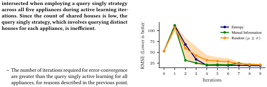
The paper's central claim is that uncertainty-based active learning can identify the subset of households whose appliance-level data is most valuable for training NILM models. On a public residential energy dataset with five appliances, the authors report that entropy and mutual-information acquisition functions both outperform random sampling; mutual information is particularly effective for appliances that are used rarely and irregularly, such as dishwashers and clotheswashers. They report that roughly 30% of the labeled data suffices to match the accuracy of a model trained on the full pool, and that for a fixed number of installed sensors the strategy reduces root mean squared error by up to a factor of two in the early iterations of active learning.
Load-bearing premise
The active learning scores each candidate house using a seven-day window of future mains data; if that future data is not available at query time, the advantage over random may shrink or vanish.
Editorial extensions
If this is right
- If the claim holds, energy utilities can install appliance monitors in only about 30% of homes and still train disaggregation models that match full-data performance, cutting sensor hardware and installation cost substantially.
- For sparsely used appliances, acquisition functions based on mutual information (epistemic uncertainty) are more cost-efficient than entropy-based ones, because they avoid spending budget on houses whose data noise is high.
- For seasonally varying appliances, scoring houses over a dynamic recent window (as opposed to a fixed past window) yields better models, because it tracks the appliance's current usage regime.
- Jointly querying a single house for all appliances ('query all at once') is a practical approximation: it requires more sensors than the per-appliance ideal, but still considerably fewer than random selection, e.g., four sensors instead of eight for air conditioners.
Reading between the lines
- The reported advantage is measured under a look-ahead: each house's uncertainty score uses seven days of future mains data, which is unavailable at query time in practice. A corrected protocol that uses only past data (or previous-year data as a proxy) is the natural next test, and could shrink the gap.
- The same uncertainty-guided sensor placement logic could transfer to other building-level metering tasks—water, gas, or room-level electricity—where a cheap aggregate signal is available but per-device instrumentation is expensive.
- The query-singly results show near-zero overlap in selected houses across appliances in early iterations, implying that a single fixed house rarely dominates uncertainty for all appliances; a batch-selection method that accounts for shared information across houses could recover some of the per-appliance gains in the practical query-all-at-once setting.
- A stopping criterion based on uncertainty (when the acquisition score falls below a threshold) could further reduce sensor count; the paper lists this as future work, but the reported error curves suggest diminishing returns after the first few queries.
Editorial analysis
A structured set of objections, weighed in public.
Referee Report
Summary. The paper proposes an active learning framework for non-intrusive load monitoring (NILM), in which a model actively selects houses to instrument with appliance-level sensors. The authors build on Seq2Point networks with heteroskedastic outputs and MC-dropout uncertainty, and compare entropy and mutual-information acquisition functions against a random baseline and a full-data 'total' baseline. Experiments on Pecan Street Dataport cover a single-appliance ('query singly') setting and a multi-appliance ('query all at once') setting, using static and dynamic temporal pooling. The headline claims are that active learning matches full-data performance with roughly 30% of the data and reduces disaggregation error by up to 2x relative to random. The manuscript includes code and is framed as a benchmark.
Significance. If the empirical claims survive a causally correct evaluation, this would be a useful contribution to NILM and to active learning for time-series regression. The paper is clearly written, uses a public dataset, reports a random baseline over 10 seeds, and evaluates two standard acquisition functions. However, the main result currently relies on a dynamic pool window that uses future mains data at acquisition time, which is not available in any real deployment; until this is corrected, the central comparison is not trustworthy. The paper also lacks repeated runs of the AL methods themselves, so the claimed 'significant' improvement over random is not statistically quantified. These issues are fixable within the manuscript's scope, which is why I recommend major revision rather than rejection.
major comments (3)
- [§5.3.7 and Eq. (14)] The dynamic pool window includes T+7 days of future mains data when scoring pool-house uncertainty. At query time, this future data is unavailable, and the paper itself concedes in §5.3.7 that 'we will never have access to future data for evaluating pool uncertainty.' More seriously, because the final acquisition iterations occur in late April, the T+7 window overlaps the May 1–10 test period, so the acquisition function uses test-period mains data for pool houses. All headline results (Figures 6–14 and the abstract claims of '2x reduction' and '~30% data') use this dynamic triangle-weighted window. The static-window comparisons in Figures 7–8 do not repair this, since they are not the basis of the headline claims. Please re-run the experiments with a causal window (e.g., T−14 to T, or previous-year data as suggested in §5.3.7) and report whether the advantage over random persists. Without this, the central empirical claim is not established.
- [§5.4.1, Figures 6–14] The active-learning acquisition curves (entropy and MI) are presented as single runs, while only the random baseline is repeated across 10 seeds and shown as mean ± σ. The text states that the AL results are 'well below the sigma interval' of random, but without repeated AL runs or a statistical test, the claim that AL 'significantly outperforms' random is not fully supported. Please provide multiple seeds (or at least confidence intervals) for the AL strategies, or a paired significance test across the same random seeds.
- [§5.4.2] The query-all-at-once setting, which the paper argues is the realistic one, does not include a total baseline ('Due to resource constraints, we have not evaluated the total baseline error for query all at once AL'). Therefore the abstract's claim of achieving 'performance comparable to models trained on the entire dataset' is only demonstrated in the query-singly setting, which the paper itself shows is impractical because different appliances select different houses (Figure 9). Please either add the total baseline to the query-all-at-once experiments or restrict the comparable-to-full-data claim accordingly.
minor comments (5)
- [§5.3.4 vs §5.3.7] There is a small inconsistency in the start date of the first acquisition: §5.3.4 says 'starting from 11 March 2018', while §5.3.7 says 'the dynamic window starts from 5−20 March 2018'. Please clarify whether the first query occurs on 11 March and how the dynamic window is centered on that date.
- [§4.2.1, Eq. (6)] Equation (6) approximates the differential entropy of the predictive mixture by log(σ_ensemble) plus a constant, but for a Gaussian mixture (Eq. (1)) the entropy is not exactly that of the single Gaussian with the aggregate variance; there is an additional term due to the spread of component means. Please state that this is an approximation and, if possible, assess its effect on acquisition rankings.
- [§2.2.3 and §4.2.2] The notation around Eqs. (1), (9), and (10) is confusing: the mixture components are written as N(x | μ_i, σ_i) but the variable being predicted is y, and x_s is used both as a sample and as the conditioning input. Please make the distinction between input and output variables consistent.
- [§5.1] Typos: 'Additionaly' should be 'Additionally' in Section 5.1; §5.3.6 contains 'i.e i.e.' with a missing comma; §5.3.8 says 'we use4 X NVidia A100 GPUs' (missing space). Please update these.
- [§5.3.7] The sentence 'For the purposes of a practical implementation, one could use the data from the previous year (if available) or introduce a lag in adding pool data (till the end of the pool window)' actually describes the correct causal protocol, but no such evaluation is reported. Highlighting the corrected protocol in the main results would strengthen the paper.
Circularity Check
No circularity: the active-learning acquisition functions and the held-out test evaluation are independent of the reported performance gains.
full rationale
The paper's central claim is an empirical comparison, not a derivation that reduces to its own inputs. The acquisition functions in Section 4.2 (Eq. 6 for entropy and Eq. 7 for mutual information) are standard estimators built from the MC-dropout predictive distribution (Eqs. 1-3); house selection via Eq. 4 maximizes one of these acquisition values over the pool. The evaluation metric in Eq. 13 is RMSE on test houses that are disjoint from train and pool houses (Section 5.3.2), and the test period (May 1-10, Section 5.3.5) is not used to choose acquisitions. Consequently, the reported '~30% of the data' and '2x reduction' results are empirical outcomes rather than identities forced by definition. The self-citations ([2] for heteroskedastic S2P uncertainty, [31] for the train/test split) supply setup choices but not the comparative result against random sampling, so they are not load-bearing circularity. The dynamic pool window in Section 5.3.7 includes T+7 future mains days, and the paper itself concedes this is unavailable in practice; that is a temporal-leakage and protocol concern about the comparison's validity, not a case where the claimed prediction is equivalent to the acquisition input. No circular step is identified.
Assumptions & free parameters
free parameters (4)
- F (MC dropout forward passes) =
not reported in paper; linked in placeholder repo
- S (Monte Carlo samples for MI) =
not reported in paper
- MC dropout rate =
not reported in paper
- Dynamic window half-width and triangle kernel divisor =
k=7 days; divisor 8 in Eq. 14
assumptions (4)
- domain assumption MC dropout with F stochastic passes yields a calibrated approximation of the Bayesian posterior predictive distribution.
- domain assumption Appliance power at a given time follows a heteroskedastic Gaussian distribution with input-dependent mean and sigma.
- domain assumption The fixed 5-train / 5-test / 10-pool house split from prior literature [31] and the March-May 2018 window are representative for comparing query strategies.
- ad hoc to paper Future mains data (up to T+7 days) can be included in the acquisition score at time T.
Cite this review
Pith. "Pith review of Benchmarking Active Learning for NILM." pith.science (2026). https://pith.science/paper/22QTTJBS
@misc{pith2026241115805,
  author       = {Pith},
  title        = {Pith review of: Benchmarking Active Learning for NILM},
  year         = {2026},
  howpublished = {\url{https://pith.science/paper/22QTTJBS}},
  note         = {Machine review of arXiv:2411.15805}
}
read the original abstract
Non-intrusive load monitoring (NILM) focuses on disaggregating total household power consumption into appliance-specific usage. Many advanced NILM methods are based on neural networks that typically require substantial amounts of labeled appliance data, which can be challenging and costly to collect in real-world settings. We hypothesize that appliance data from all households does not uniformly contribute to NILM model improvements. Thus, we propose an active learning approach to selectively install appliance monitors in a limited number of houses. This work is the first to benchmark the use of active learning for strategically selecting appliance-level data to optimize NILM performance. We first develop uncertainty-aware neural networks for NILM and then install sensors in homes where disaggregation uncertainty is highest. Benchmarking our method on the publicly available Pecan Street Dataport dataset, we demonstrate that our approach significantly outperforms a standard random baseline and achieves performance comparable to models trained on the entire dataset. Using this approach, we achieve comparable NILM accuracy with approximately 30% of the data, and for a fixed number of sensors, we observe up to a 2x reduction in disaggregation errors compared to random sampling.
Figures


Figures from the paper (10 more)




Reference graph
Works this paper leans on
-
[1]
A mathematical theory of communication
1948. A mathematical theory of communication. The Bell system technical journal 27, 3 (1948), 379–423
work page 1948
-
[2]
Vibhuti Bansal, Rohit Khoiwal, Hetvi Shastri, Haikoo Khandor, and Nipun Batra. 2022. " I do not know" quantifying uncertainty in neu- ral network based approaches for non-intrusive load monitoring. In Proceedings of the 9th ACM International Conference on Systems for Energy-Efficient Buildings, Cities, and Transportation . 79–88
work page 2022
-
[3]
Nipun Batra, Jack Kelly, Oliver Parson, Haimonti Dutta, William Knot- tenbelt, Alex Rogers, Amarjeet Singh, and Mani Srivastava. 2014. NILMTK: An open source toolkit for non-intrusive load monitoring. In Proceedings of the 5th international conference on Future energy systems . 265–276
work page 2014
-
[4]
Nipun Batra, Rithwik Kukunuri, Ayush Pandey, Raktim Malakar, Ra- jat Kumar, Odysseas Krystalakos, Mingjun Zhong, Paulo Meira, and Oliver Parson. 2019. A demonstration of reproducible state-of-the-art energy disaggregation using NILMTK. In Proceedings of the 6th ACM international conference on systems for energy-efficient buildings, cities, and transportat...
work page 2019
-
[5]
Charles Blundell, Julien Cornebise, Koray Kavukcuoglu, and Daan Wierstra. 2015. Weight uncertainty in neural network. In International conference on machine learning . PMLR, 1613–1622
work page 2015
-
[6]
David A Cohn, Zoubin Ghahramani, and Michael I Jordan. 1996. Ac- tive learning with statistical models. Journal of artificial intelligence research 4 (1996), 129–145
work page 1996
-
[7]
Yarin Gal and Zoubin Ghahramani. 2016. Dropout as a bayesian approximation: Representing model uncertainty in deep learning. In international conference on machine learning . PMLR, 1050–1059
2016
-
[8]
Yarin Gal, Riashat Islam, and Zoubin Ghahramani. 2017. Deep bayesian active learning with image data. InInternational conference on machine learning. PMLR, 1183–1192
work page 2017
Show all 41 references
-
[9]
Piotr Garbaczewski. 2006. Differential entropy and dynamics of uncer- tainty. Journal of Statistical Physics 123 (2006), 315–355
2006
-
[10]
Luyang Guo, Shouxiang Wang, Haiwen Chen, and Qingyuan Shi. 2020. A Load Identification Method Based on Active Deep Learning and Discrete Wavelet Transform. IEEE Access 8 (2020), 113932–113942. https://doi.org/10.1109/ACCESS.2020.3003778
2020
-
[11]
George William Hart. 1992. Nonintrusive appliance load monitoring. Proc. IEEE 80, 12 (1992), 1870–1891
1992
-
[12]
W Keith Hastings. 1970. Monte Carlo sampling methods using Markov chains and their applications. (1970)
1970
-
[13]
Manuel Haußmann, Fred A Hamprecht, and Melih Kandemir. 2020. Sampling-free variational inference of bayesian neural networks by variance backpropagation. In Uncertainty in Artificial Intelligence . PMLR, 563–573
2020
-
[14]
Kanghang He, Lina Stankovic, Jing Liao, and Vladimir Stankovic. 2016. Non-intrusive load disaggregation using graph signal processing. IEEE Transactions on Smart Grid 9, 3 (2016), 1739–1747
2016
- [15]
-
[16]
Patrick Huber, Alberto Calatroni, Andreas Rumsch, and Andrew Paice
-
[17]
Jie Jiang, Qiuqiang Kong, Mark D Plumbley, Nigel Gilbert, Mark Hoogendoorn, and Diederik M Roijers. 2021. Deep learning-based energy disaggregation and on/off detection of household appliances. ACM Transactions on Knowledge Discovery from Data (TKDD) 15, 3 (2021), 1–21
2021
-
[18]
Jack Kelly and William Knottenbelt. 2015. Neural nilm: Deep neural networks applied to energy disaggregation. In Proceedings of the 2nd Conference acronym ’XX, June 03–05, 2018, Woodstock, NY Dhruv Patel, Ankita Kumari Jain, Haikoo Khandor, Xhitij Choudhary, Nipun Batra ACM in...
2015
-
[19]
Andreas Kirsch, Joost Van Amersfoort, and Yarin Gal. 2019. Batch- bald: Efficient and diverse batch acquisition for deep bayesian active learning. Advances in neural information processing systems 32 (2019)
2019
-
[20]
J Zico Kolter, Siddharth Batra, and Andrew Y Ng. 2010. Energy dis- aggregation via discriminative sparse coding. In Advances in Neural Information Processing Systems. 1153–1161
2010
-
[21]
J Zico Kolter and Tommi Jaakkola. 2012. Approximate inference in additive factorial hmms with application to energy disaggregation. In Artificial intelligence and statistics. 1472–1482
2012
-
[22]
Solomon Kullback and Richard A Leibler. 1951. On information and sufficiency. The annals of mathematical statistics 22, 1 (1951), 79–86
1951
-
[23]
Balaji Lakshminarayanan, Alexander Pritzel, and Charles Blundell
-
[24]
Peter D Lund, Juuso Lindgren, Jani Mikkola, and Jyri Salpakari. 2015. Review of energy system flexibility measures to enable high levels of variable renewable electricity. Renewable and sustainable energy reviews 45 (2015), 785–807
2015
-
[25]
Radford M Neal et al . 2011. MCMC using Hamiltonian dynamics. Handbook of markov chain monte carlo 2, 11 (2011), 2
2011
-
[26]
Oliver Parson, Grant Fisher, April Hersey, Nipun Batra, Jack Kelly, Amarjeet Singh, William Knottenbelt, and Alex Rogers. 2015. Dataport and NILMTK: A building data set designed for non-intrusive load monitoring. In 2015 IEEE Global Conference on Signal and Information Process...
2015
-
[27]
Oliver Parson, Siddhartha Ghosh, Mark Weal, and Alex Rogers. 2012. Non-Intrusive Load Monitoring Using Prior Models of General Ap- pliance Types. In Proceedings of the Twenty-Sixth AAAI Conference on Artificial Intelligence (Toronto, Ontario, Canada) (AAAI’12). AAAI Press, 356–362
2012
-
[28]
Christian P Robert, George Casella, and George Casella. 1999. Monte Carlo statistical methods. Vol. 2. Springer
1999
-
[29]
Greg Schohn and David Cohn. 2000. Less is more: Active learning with support vector machines. In ICML, Vol. 2. Citeseer, 6
2000
-
[30]
Burr Settles. 2009. Active learning literature survey. (2009)
2009
-
[31]
Hetvi Shastri and Nipun Batra. 2021. Neural Network Approaches and Dataset Parser for NILM Toolkit. In Proceedings of the 8th ACM International Conference on Systems for Energy-Efficient Buildings, Cities, and Transportation (Coimbra, Portugal) (BuildSys ’21). Asso- ciation fo...
2021
-
[32]
Nitish Srivastava, Geoffrey Hinton, Alex Krizhevsky, Ilya Sutskever, and Ruslan Salakhutdinov. 2014. Dropout: a simple way to prevent neural networks from overfitting. The journal of machine learning research 15, 1 (2014), 1929–1958
2014
-
[33]
Luke Tierney and Joseph B Kadane. 1986. Accurate approximations for posterior moments and marginal densities. Journal of the american statistical association 81, 393 (1986), 82–86
1986
-
[34]
Tamara Todic, Vladimir Stankovic, and Lina Stankovic. 2023. An active learning framework for the low-frequency Non-Intrusive Load Monitoring problem. Applied Energy 341 (2023), 121078. https://doi. org/10.1016/j.apenergy.2023.121078
2023
-
[35]
Evgenii Tsymbalov, Maxim Panov, and Alexander Shapeev. 2018. Dropout-based active learning for regression. InAnalysis of Images, So- cial Networks and Texts: 7th International Conference, AIST 2018, Moscow, Russia, July 5–7, 2018, Revised Selected Papers 7 . Springer, 247–258
2018
-
[36]
Joost Van Amersfoort, Lewis Smith, Yee Whye Teh, and Yarin Gal
-
[37]
Donggeun Yoo and In So Kweon. 2019. Learning loss for active learning. In Proceedings of the IEEE/CVF conference on computer vision and pattern recognition. 93–102
2019
-
[38]
Chaoyun Zhang, Mingjun Zhong, Zongzuo Wang, Nigel Goddard, and Charles Sutton. 2018. Sequence-to-point learning with neural networks for non-intrusive load monitoring. In Thirty-second AAAI conference on artificial intelligence
2018
-
[2017]
Advances in neural information processing systems 30 (2017)
Simple and scalable predictive uncertainty estimation using deep ensembles. Advances in neural information processing systems 30 (2017)
2017
-
[2020]
In International conference on machine learning
Uncertainty estimation using a single deep deterministic neural network. In International conference on machine learning . PMLR
-
[2021]
Energies 14, 9 (2021), 2390
Review on deep neural networks applied to low-frequency nilm. Energies 14, 9 (2021), 2390
2021
Reviewed August 12, 2026 · model on record in the stance chip above.
Discussion (0). Continue with ORCID to comment.