REVIEW 3 major objections 4 minor 21 references
Entangling color centers via magnon-antimagnon pair creation
T0 review · 3 major / 4 minor · reviewed 2026-08-12 · deepseek-v4-flash
Pith's one-line read Two weakly coupled color centers can reach a near-maximally entangled steady state through magnon-antimagnon pair creation at a ferromagnet interface.
desk verdict Genuinely new dissipative-entanglement proposal built on the magnonic Klein paradox; the unquantified neglect of the stabilizing spin torque in the scattering amplitudes is the main thing to fix. read the letter →
The pith
A machine-rendered reading of the paper's core claim, the machinery that carries it, and where it could break.
The reading
What carries the argument
The load-bearing object is the two-mode squeezing of positive-energy magnons on the left and negative-energy antimagnons on the right, encoded in a generalized nonunitary scattering theory in bosonic Bogoliubov space. The scattering matrix satisfies $S\Sigma S^\dagger = \Sigma$ and yields the identity $|r|^2 - |t|^2 = 1$, which lies at the heart of the bosonic Klein paradox and directly controls the pair-creation rate. The second essential element is the chiral magnetostatic coupling between the color centers and the magnon stray field: it guarantees $h_s^z = 0$, eliminating magnon-induced dephasing, and it makes each color center sensitive only to magnons moving in one direction, so that the position dependence drops out and the dynamics are captured by just two Lindblad operators $L_1$ and $L_2$ describing nonlocal emission and absorption.
What would settle it
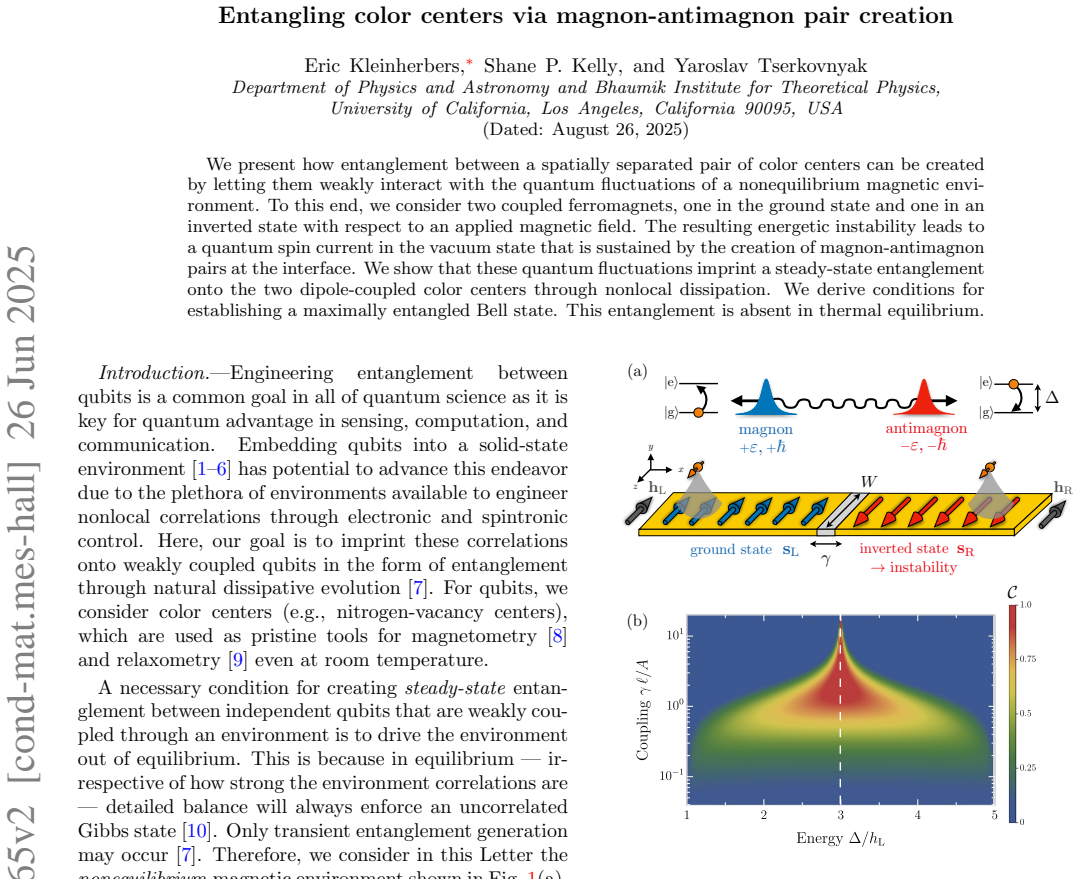
A direct test would place two color centers at height $d$ on opposite sides of the interface, tune their energy splitting $\Delta$ through $(h_L+h_R)/2$, and perform two-qubit state tomography on the steady state; the paper predicts concurrence $C = 2rt/(r^2+t^2)$ rising toward one with interfacial coupling, so observing $C = 0$ across all $\Delta$ and $\gamma$ would falsify the central claim.
Extended reading notes
Core claim
The paper's discovery is a dissipative entanglement-creation mechanism that requires no external drive on the two qubits: the energy needed for pair creation is supplied by the inverted ferromagnet, and the interfacial exchange coupling merely acts as an outlet that harvests the instability. The pair-creation amplitudes obey the bosonic Klein-paradox identity $r^2 - t^2 = 1$, so the reflected magnon amplitude is enhanced beyond unity, with the excess accounted for by the antimagnon transmitted into the inverted region. When two color centers are chirally coupled to the stray field on opposite sides of the interface, the master equation reduces to two Lindblad operators, and at the tuned energy $\Delta = (h_L+h_R)/2$ the steady state becomes pure with concurrence $C = 2rt/(r^2+t^2)$. In the limit $r \approx t \gg 1$, this state approaches the Bell state $(\lvert g,e\rangle - \lvert e,g\rangle)/\sqrt{2}$.
Load-bearing premise
The load-bearing premise is that a spin torque can hold the inverted ferromagnet in its inverted vacuum state, with stability condition $-\hbar\Delta_s > \alpha h_R$, without modifying the magnon scattering amplitudes from which the pair creation and Lindblad operators are derived.
Editorial extensions
If this is right
- Steady-state entanglement is generated without coherent driving of the qubits, because the inverted ferromagnet acts as the energy source; two color centers placed on opposite sides of the interface should become entangled after a relaxation time set by $\Gamma_0$.
- At the resonance $\Delta = (h_L+h_R)/2$ and with interfacial coupling tuned so that $r \approx t$, the steady state approaches the Bell state $(\lvert g,e\rangle - \lvert e,g\rangle)/\sqrt{2}$, with concurrence $C = 2rt/(r^2+t^2)$ tending to one.
- The effect is a genuine nonequilibrium resource: in thermal equilibrium detailed balance enforces an uncorrelated Gibbs state, so the same geometry would show no steady-state entanglement.
- The enhanced reflection $r > 1$ manifests as a purely quantum spin current flowing to the left in the vacuum state, so detecting that current at zero temperature is a direct signature that magnon-antimagnon pairs are being created at the interface.
Reading between the lines
- Editorial inference: the same interface could serve as an on-chip entanglement source for nitrogen-vacancy or similar color centers without microwave driving, requiring only that the centers be placed near the ferromagnetic strip and their energy $\Delta$ tuned through an external field; a two-qubit state tomography experiment at the sweet spot would directly test the predicted concurrence.
- Editorial inference: because the master equation depends only on two Lindblad operators with coefficients $r$ and $t$, any two-level systems coupled chirally to the stray field should inherit the same steady-state entanglement, suggesting extensions to other solid-state qubits or molecular magnets that the paper does not explicitly explore.
- Editorial inference: the non-monotonic dependence of concurrence on the interfacial coupling $\gamma$ is a sharp falsifiable prediction; if entanglement keeps growing monotonically with $\gamma$ beyond the predicted sweet spot $\gamma \sim \sqrt{A(h_R-h_L)}$, the scattering treatment would need revision.
Signed reviews
Editorial analysis
A structured set of objections, weighed in public.
Referee Report
Summary. The paper proposes a scheme to entangle two color centers by placing them in the stray field of a nonequilibrium magnetic environment: a ground-state ferromagnet coupled at an interface to an inverted-state ferromagnet that is dynamically stabilized by spin torque. Quantum fluctuations at the interface create magnon-antimagnon pairs, sustaining a quantum spin current. The authors derive a Lindblad master equation for the color centers, with nonlocal dissipation governed by the pair-creation amplitudes r and t, and show that at the resonant energy Delta = (h_L + h_R)/2 the steady state is a pure entangled state of the form (r|g,e> - t|e,g>)/sqrt(r^2+t^2), approaching a Bell state when r ~ t. The derivation combines a bosonic Bogoliubov scattering calculation for the magnon field, a magnetostatic Green's-function treatment of the stray field, and a numerical concurrence plot.
Significance. If the result holds, the paper provides a new mechanism for steady-state entanglement of solid-state spin qubits using a magnetic environment that is not in thermal equilibrium, with no parametric drive applied directly to the qubits. The main strengths are that the scattering amplitudes are derived from the interface exchange coupling rather than fitted, the Lindblad operators are obtained from the magnetostatic Green's functions, the chiral nature of the coupling is shown to eliminate dephasing, and the steady-state expression is explicit. The proposal is conceptually interesting and could be relevant for quantum spintronics and dissipative entanglement engineering. The principal weakness is that the central operating point relies on a spin-torque-stabilized inverted magnet, while the scattering calculation neglects that stabilization; quantitative control of this approximation is missing, so the near-unit-concurrence sweet spot is not yet fully secured.
major comments (3)
- [Supplement I.B.1-I.B.2; main text 'Nonequilibrium magnetic environment'] The inverted ferromagnet is defined as a spin-torque-stabilized nonequilibrium state in Supplement Eqs. (2)-(3), with stability condition -hbar Delta_s > alpha h_R, but the scattering calculation of the pair-creation amplitudes r and t is then performed for the undriven, dissipationless system, as stated in Supplement I.B.2: 'we neglect dissipation and driving in the following'. The amplitudes in Eqs. (30)-(31) and (35)-(36), and hence the Lindblad operators in Eqs. (12)-(13) of the main text, are those of the idealized inverted magnet rather than of the stabilized driven magnet. Unless the residual damping gamma_d = -hbar Delta_s - alpha h_R is infinitesimal, the right-side BdG Hamiltonian acquires an imaginary part, right-moving antimagnons acquire a finite decay length, and the scattering amplitudes change, altering t/r and the resonance condition. The spin-torque reservoir also carries its own noise, which is not included in the vacuum correlators used to derive the master equation. The paper does not provide a small-parameter estimate for these corrections, so the existence of the near-unit-concurrence sweet spot is not yet secured.
- [Supplement II.B; Eq. (11)] The Lindblad master equation (11) is derived in a Born-Markov approximation, but no dimensionless small parameter is identified. The rate Gamma_0 = mu_e^4 hbar^2 s / (W^2 A d) is quoted, yet the conditions under which this rate is small compared with the relevant energy scales (e.g., Delta, h_R - h_L) or with the inverse environment correlation time are not given. Since the environment is gapless and the steady-state concurrence is obtained from this master equation, the paper should state the explicit weak-coupling regime in which the Born-Markov treatment is controlled.
- [Supplement II.B.2; footnote [30]] The environment-induced local Lamb shift proportional to delta_alpha sigma^z_alpha is acknowledged but not computed, and the paper notes that the dynamics is sensitive to delta_L - delta_R. The resonant sweet spot is tuned to Delta = (h_L + h_R)/2, so an unquantified difference delta_L - delta_R could shift or disrupt the optimal condition. The authors should provide an estimate or a symmetry argument showing that delta_L = delta_R (or that the difference is negligible compared with the relevant linewidth), otherwise the claimed resonance condition is not fully determined.
minor comments (4)
- [Main text, Eq. (3) and surrounding text] The interfacial coupling is denoted gamma in Eq. (3) and Fig. 1(b), but later the text refers to 'mu -> 0' and 'mu > 0' for the same quantity; this notation should be unified, or the mapping between gamma and the Supplement's mu should be stated explicitly.
- [Fig. 1(b)] The color map for the concurrence C has no colorbar or numerical scale, making it difficult to read the claimed values close to one; please add a colorbar.
- [Supplement I.A, mapping table] The operator b^dagger_{-epsilon} appears in the mapping between the Letter and Supplement notation but is not defined in the main text; please define all operators and the vacuum state explicitly.
- [Supplement II.A, Eq. (65)] The expression for the spin density per volume, Theta(|z| - W/2)/W, appears dimensionally unusual; please verify the normalization and clarify the role of the width W.
Circularity Check
No significant circularity: the predicted entanglement is derived from interface scattering amplitudes and magnetostatic Green's functions, not from fitting or from a load-bearing self-citation.
full rationale
The derivation chain is self-contained. The scattering amplitudes r and t are computed from the interfacial exchange Hamiltonian via a bosonic Bogoliubov matching calculation (Supplement Eqs. (30)-(31), (35)-(36)), with r^2 - t^2 = 1 following from the nonunitary scattering structure; they are not fitted parameters chosen to produce entanglement. The Lindblad operators L1 and L2 are obtained by evaluating stray-field Green's functions in the scattering vacuum (Supplement Eqs. (74)-(83)), and the Bell-like steady state at Delta=(hL+hR)/2, |psi>=(r|g,e>-t|e,g>)/sqrt(r^2+t^2), is a derived fixed point of that master equation, not an input. The concurrence formula C=2rt/(r^2+t^2) is then a standard evaluation for that pure state. The self-citations, e.g., Ref. [7] for dissipative coupling and the methodological follow-up in the supplement, are used as framework references with stated assumptions that do not include the target Bell-state result, and the key steps are re-derived in the paper. The one explicit limitation is in Supplement I.B.2, where the authors introduce spin-torque stabilization and then state 'we neglect dissipation and driving in the following'; this is a model-consistency and correctness concern about whether the stabilizing drive modifies the pair-creation amplitudes, but it is not a circular reduction, because the scattering amplitudes are not defined in terms of the claimed entanglement outcome. Overall, no step in the claimed derivation reduces to its own inputs or to a fitted parameter renamed as a prediction.
Assumptions & free parameters
assumptions (6)
- domain assumption Linearized Holstein-Primakoff description of spin fluctuations in the large-spin limit.
- domain assumption The inverted magnet can be maintained in its inverted vacuum state by spin-transfer torque despite its energetic instability.
- domain assumption Born-Markov and secular approximations are valid for integrating out the magnetic environment.
- domain assumption The magnetostatic stray field can be approximated by the two-dimensional limit d << W with |x_alpha| >> d, giving a chiral field with hz_s = 0.
- domain assumption The higher-energy scattering solution a3 does not resonantly couple to the color centers and can be dropped in the secular approximation.
- domain assumption Local Lamb shifts renormalize the color-center energies and can be ignored because only the difference delta_L - delta_R matters.
Cite this review
Pith. "Pith review of Entangling color centers via magnon-antimagnon pair creation." pith.science (2026). https://pith.science/paper/TYCMIYNT
@misc{pith2026241109865,
  author       = {Pith},
  title        = {Pith review of: Entangling color centers via magnon-antimagnon pair creation},
  year         = {2026},
  howpublished = {\url{https://pith.science/paper/TYCMIYNT}},
  note         = {Machine review of arXiv:2411.09865}
}
read the original abstract
We present how entanglement between a spatially separated pair of color centers can be created by letting them weakly interact with the quantum fluctuations of a nonequilibrium magnetic environment. To this end, we consider two coupled ferromagnets, one in the ground state and one in an inverted state with respect to an applied magnetic field. The resulting energetic instability leads to a quantum spin current in the vacuum state that is sustained by the creation of magnon-antimagnon pairs at the interface. We show that these quantum fluctuations imprint a steady-state entanglement onto the two dipole-coupled color centers through nonlocal dissipation. We derive conditions for establishing a maximally entangled Bell state. This entanglement is absent in thermal equilibrium.
Figures


Figures from the paper (7 more)


Reference graph
Works this paper leans on
-
[1]
( 10)-(11) to a classical scattering problem, we insert Eq
Classical scattering problem To reduce the field operator equations from Eq. ( 10)-(11) to a classical scattering problem, we insert Eq. ( 12) and apply the commutator from Eq. ( 13) to obtain εφ L,i = HBdG L φL,i, for x< 0, (15) εφ R,i = HBdG R φR,i, for x> 0, (16) 2 Since ψ L(x) and ψ L(x) are only defined for x ≤ 0 and x ≥ 0, respectively, the action of ...
-
[2]
Exchange coupling at interface At the interface, both magnets are coupled via exchange interaction HI = ˜µ¶(x)sL · sR ≈µ¶(x) ( È LÈL +È RÈR +ÈLÈR +È LÈ R ) , (9) 4 where we, again, rescale the coupling parameter through µ = ℏs˜µ.2 The sign of µ can be either ferromagnetic or antiferromagnetic. Crucially, this coupling contains terms of the for m ∼ ¶(x)È L...
-
[3]
Here, mα, ± and ¯mα, ± are the four eigenmodes of the bulk equations Eq
Ansatz for scattering solution To find the scattering solutions, we use the ansatz φα,i =aα,i mα, + +bα,i mα, − + ¯aα,i ¯mα, + + ¯bα,,i ¯mα, −, (21) where aα,i , ¯aα,i ,b α,i and ¯bα,i are the energy-dependent scattering amplitudes and i labels the different scattering solutions. Here, mα, ± and ¯mα, ± are the four eigenmodes of the bulk equations Eq. ( 15)...
-
[4]
Matching of scattering amplitudes To obtain the energy-dependent scattering amplitudes aα,i , ¯aα,i ,b α,i and ¯bα,i of the scattering solution Eq. ( 21), we use the boundary condition to link the amplitudes on the left and right side of the interface via aL,i bL,i ¯aL,i ¯bL,i = M aR,i bR,i ¯aR,i ¯bR,i . (26) The transfer matrix is ...
-
[5]
Inscattering states The matching conditions given by Eq. ( 26) have to be complemented with scattering boundary conditions. Here , we construct the inscattering states φin α,i of the problem, where a plane-wave mode m α, ± or ¯mα, ± with amplitude 1 is impinging on the interface and gets scattered into the outgoing plane -wave modes. The number of possibl...
-
[6]
Scattering matrix To define the scattering matrix S, we write the three scattering solutions from Sec. I C 4 a- I C 4 c via φ in 1 φ in 2 φ in 3 = m L, + ¯mR, − mR, − + r1 ¯t1 0 t2 ¯r2 0 0 0 r3 /bracehtipupleft /bracehtipdownright/bracehtipdownleft/bracehtipupright =ST m L, − ¯mR, + mR, + , (50) where we used the notation φ i...
-
[7]
W. K. Wootters, Entanglement of formation of an arbitrary state of two qubits, Phys. Rev. Lett. 80, 2245 (1998)
1998
-
[8]
Two-mode squeezing The relation between ain 1, 2 and aout 1, 2 from Eq. (
Show all 21 references
-
[12]
Dissipative coupling For the dissipative coupling, we obtain Γ = Γ 1 · Γ 2 = 1 4 iG > LL iG > LR 0 0 iG > RL iG > RR 0 0 0 0 iG < LL iG < RL 0 0 iG < LR iG < RR , (73) where the 1 /4 originates from the coupling Hamiltonian from Eq. ( 63). The ℏ cancels in the deriv...
-
[13]
(85) Here we followed Ref
Coherent coupling Besides the dissipative coupling, the environment generically als o mediates a nonlocal coherent coupling similar to RKKY interaction of the form ¶H =JÃ + LÃ− R +J ∗Ã+ RÃ− L, (84) where J = 1 4 ReGR RL(∆) . (85) Here we followed Ref. [ 6] and defined a “real” ...
-
[15]
J. S. Harms, H. Y. Yuan, and R. A. Duine, Antimagnonics, AIP Adv. 14, 025303 (2024)
2024
-
[16]
Balbinot, I
R. Balbinot, I. Carusotto, A. Fabbri, C. Mayoral, and A. Reca ti, Understanding Hawking radiation from simple models of atomic Bose-Einstein condensates, in Analogue Gravity Phenomenology: Analogue Spacetimes and H orizons, from Theory to Experiment, edited by D. Faccio, F. Be...
2013
-
[17]
G. B. Lesovik and I. A. Sadovskyy, Scattering matrix approac h to the description of quantum electron transport, Phys.- Uspekhi 54, 1007 (2011)
2011
-
[18]
K. Y. Guslienko and A. N. Slavin, Magnetostatic Green’s fun ctions for the description of spin waves in finite rectangular magnetic dots and stripes, J. Magn. Magn. Mater. 323, 2418 (2011)
2011
-
[19]
Halbach, Application of permanent magnets in accelerat ors and electron storage rings, J
K. Halbach, Application of permanent magnets in accelerat ors and electron storage rings, J. Appl. Phys. 57, 3605 (1985)
1985
-
[20]
J. Zou, S. Zhang, and Y. Tserkovnyak, Bell-state generatio n for spin qubits via dissipative coupling, Phys. Rev. B 106, L180406 (2022)
2022
-
[52]
( 54) yields the relations t2 = −¯t1 andt∗ 2 ¯r2 = ¯t1r∗ 1 as well as |r1|2 − |¯t1|2 = 1 and |¯r2|2 − |t2|2 = 1
and Eq. ( 54) yields the relations t2 = −¯t1 andt∗ 2 ¯r2 = ¯t1r∗ 1 as well as |r1|2 − |¯t1|2 = 1 and |¯r2|2 − |t2|2 = 1. (55)
-
[53]
dDmzny9W/9WHEBFFMZSVNLMDXgc=
given by the scattering matrix S can also be formulated in Fock space using a two-mode squeezing transformation U such that e−iφ 1aout 1 =U ain 1U = coshra in 1 −e+iθ sinhra in 2, (56) e−iφ 2aout 2 =U ain 2U = coshra in 2 −e−iθ sinhra in 1, (57) where we defined cosh( r) = |r1|...
-
[54]
Thus, there is no nonlocal coherent coup ling between the color centers
for the scattering matrix. Thus, there is no nonlocal coherent coup ling between the color centers. There is, however, a local Lamb shift ∝¶αÃz α on either side, which renormalizes the bare energies ∆. This contribution will be ignored in this work as only diffe rences ¶L −¶R w...
-
[63]
Thus, the third scattering state a3 is irrelevant for the coupling in the secular approximation
gives rise to a strongly oscillating term a 3(ε)Ã− ∼ ei(ε+∆) t/ ℏ with ε >0 and ∆ > 0. Thus, the third scattering state a3 is irrelevant for the coupling in the secular approximation. B. Master equation Integrating out the environment’s degrees of freedom, we obtain the mas te...
-
[71]
In particular, the coupling term h+ s (rR)Ã− R from Eq
will not be important since it does not resonantly couple to the color centers. In particular, the coupling term h+ s (rR)Ã− R from Eq. (
Reviewed August 12, 2026 · model on record in the stance chip above.
Discussion (0). Continue with ORCID to comment.