REVIEW 5 major objections 4 minor 21 references
On-the-Go Path Planning and Repair in Static and Dynamic Scenarios
T0 review · 5 major / 4 minor · reviewed 2026-08-12 · deepseek-v4-flash
Pith's one-line read This work claims that a periodic re-planning wrapper over any static planner can guide a robot through static and dynamic obstacles by re-solving the planning problem at every distortion time T.
desk verdict Periodic replanning wrapper that violates its own stability assumption; simulations are illustrative, not evidential. read the letter →
The pith
A machine-rendered reading of the paper's core claim, the machinery that carries it, and where it could break.
The reading
What carries the argument
Algorithm 1 (the On-the-Go Motion Planning Algorithm) is the mechanism: a while loop that calls a static planner P, moves the agent to path[T], adjusts the environment, and grows T by a factor of the step counter. Algorithm 2 (a discretized planner with labeling function L and optional kinodynamic constraint handling via IsSatisfiesDynamicConstraint) serves as the concrete instantiation of P used in the experiments. The distortion time T is the pivotal quantity: it defines the re-planning horizon and must be long enough for the static planner to find a path but short enough to stay valid under the environment's dynamics.
What would settle it
Construct a scenario where a dynamic obstacle enters the agent's current cell at a time strictly less than T after the last re-plan, so the agent's position path[T] is already occupied and the next re-plan starts from a colliding state. If the planner does not detect the collision and re-route before execution, the algorithm fails to guarantee collision-free navigation, contradicting the completeness claim. A second test: in Case 4, have the adversary block the only corridor to the goal during the agent's motion and verify whether the algorithm stops with 'Road blocked completely'.
Extended reading notes
Core claim
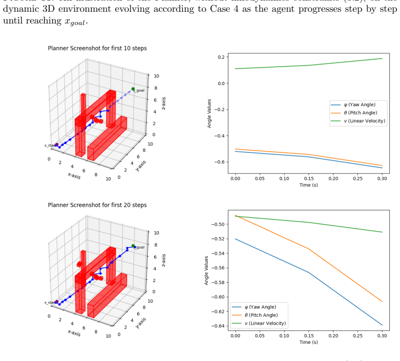
The central claim is that the temporal dynamics of the environment can be bounded by the distortion time T, and that re-planning over that window turns a deterministic static planner into a dynamic one. The paper asserts that for Cases 1 and 2 (random and disappearing obstacles) the agent always reaches the goal, while for Cases 3 and 4 (adversarial obstacles) the planner may return 'Road blocked completely' when no continuation exists. This is demonstrated in 2D and 3D experiments where the planner adjusts the initial path as new obstacles appear, with each run completing in at most 6 seconds. The completeness statement is therefore conditional: the planner seeks solutions during each distortion window, but adversarial dynamics can still cause failure.
Load-bearing premise
The environment must remain fixed for the entire distortion time T between re-planning cycles, and in the adversarial cases obstacles must never appear on the portion of the path the agent has already traversed.
Editorial extensions
If this is right
- Existing deployment of static planners in warehouses, city streets, or drone corridors can gain dynamic-obstacle handling by wrapping the planner in Algorithm 1 without changing its core.
- When the environment is genuinely stable for at least T, the agent is guaranteed to reach the goal through Cases 1 and 2, provided the underlying planner never fails.
- In adversarial environments (Cases 3 and 4), the planner explicitly returns 'Road blocked completely' when the adversary blocks all routes, providing a clean failure signal for a supervisor.
- The growth of T by a counter reduces replanning frequency over the run, which lowers computational load in calm environments.
Reading between the lines
- The scheme is a receding-horizon planner with a fixed horizon T; making T adaptive to observed change rates, or triggering re-planning on collision detection before T expires, would likely weaken Assumption 1 and improve responsiveness.
- The paper's four cases form a taxonomy of obstacle dynamics; the same wrapper could be combined with sampling-based planners (RRT, PRM) for high-dimensional spaces, though only a grid-discretized planner is tested here.
- If the static planner P is incomplete, the dynamic wrapper inherits that incompleteness; the completeness claim is therefore only as strong as the planner it wraps.
Signed reviews
Editorial analysis
A structured set of objections, weighed in public.
Referee Report
Summary. The manuscript proposes the 'On-the-Go Motion Planning Algorithm' (Algorithm 1), which wraps a static planner P in a periodic replanning loop intended for dynamic environments. Under Assumption 1, the environment is stable for a distortion time T; Algorithm 1 plans, advances the agent to path[T], adjusts the environment, and multiplies T by a counter i. Four dynamic scenarios are defined (Cases 1-4), and Algorithm 2 provides a grid-based static planner with an optional kinodynamic-constraint helper. Section 5 reports 2D and 3D simulations, but only as screenshots, and claims completeness in the distortion-time sense. The paper concludes by acknowledging that the planner may fail to reach the goal in Cases 3 and 4.
Significance. If the algorithm worked as described, a simple wrapper around a static planner would provide real-time replanning under a bounded environmental-stability assumption, which could be practically useful. The paper has some strengths: it clearly states Assumption 1, defines four dynamic scenarios, includes the implementation scripts, and explicitly acknowledges limitations in Section 6 and in the remark after Algorithm 1. However, the central guarantee in Problem 2.1 is not established: Algorithm 1 is under-specified, its progress step is undefined, and the reported validation consists of illustrative figures without quantitative metrics or comparisons to existing dynamic planners. On the evidence in the manuscript, the contribution is at best a preliminary demonstration.
major comments (5)
- [Section 2.2 / Algorithm 1, lines 8-10] The update T ← T*i violates Assumption 1. Assumption 1 guarantees stability only for the original span T, yet after the first cycle the agent is asked to follow a plan for i*T time units while the environment may change at time T. No collision check or dynamic-obstacle prediction is performed between replans, so the progress step xc ← path[T] can advance the agent into an obstacle. This is an internal contradiction, not merely a missing proof, and it undermines the central claim that Problem 2.1 is solved.
- [Algorithm 1, line 8 / Algorithm 2, line 18] path[T] is undefined. Algorithm 2 returns a discrete waypoint list traj, not a time-parameterized trajectory, while T is a real-valued time span in Assumption 1. If path is a list, path[T] with T (after the first update, a real number multiplied by i) is either an out-of-range index or a type error; if path is meant to be time-parameterized, that structure is never defined. The core update of the agent's position therefore cannot be evaluated as written.
- [Algorithm 1 and Section 5] No termination or collision-avoidance guarantee is proved. The while condition 'approximately close to xg' is informal; there is no invariant or progress measure, and the remark after Algorithm 1 explicitly allows the planner to return 'Road blocked completely.' The Section 5 statement that the planner 'exhibits completeness by actively seeking solutions within the distortion time' is not a formal completeness proof, and it equivocates: the distortion time in Assumption 1 is fixed, while Algorithm 1 multiplies it. Cases 3 and 4 additionally assume obstacles do not appear on the already covered path, but this constraint is not encoded in Algorithm 1.
- [Section 5, Figs. 3-12] The experimental validation consists entirely of screenshots. There are no quantitative metrics such as success rate, collision count, replanning frequency, or runtime per planning call, and no comparison with any baseline planner for dynamic environments. The statement that each experiment concluded in at most 6 s is not a meaningful performance measure. Consequently, the claimed effectiveness for both known and unknown environments is unsupported.
- [Section 4, helper description / Algorithm 2, line 14] The helper IsSatisfiesDynamicConstraint is assumed to return a state x' in X ∩ Φ_h(x_hat) along the agent's kinodynamic trajectory, but no argument is given that such a state exists for the chosen discretization h and the given dynamics. If no such point exists, the kinodynamic branch of Algorithm 2 cannot execute. This is load-bearing for the 3D examples with dynamics (5.2), and the assumption is stated without justification.
minor comments (4)
- [Title and running header] The title and running header contain typographical errors: 'P A TH' and 'st atic' should be corrected.
- [Algorithm 2, line 4] The labeling rule is under-specified: the quantifier over x_n is missing and the wavefront propagation condition is unclear. It should be rewritten as a standard multi-source BFS labeling.
- [Figures 5 and 6] Both captions describe the 'first scenario in Case 2'; one of them should refer to the second subcase, i.e., persistent obstacles with continuous emergence.
- [Section 6] The conclusion says the approach 'integrates a temporal dimension into the state space,' but neither Algorithm 1 nor Algorithm 2 explicitly constructs a time-augmented state space; the connection should be clarified.
Circularity Check
No circularity: the re-planning loop is validated only on the author's own simulations, but no fitted parameter, self-citation chain, or definitional identity carries the central claim.
full rationale
The paper's content is an algorithm description plus empirical simulations, not a derivation in which an output quantity is constructed from the same data it is said to predict. Algorithm 1 re-invokes a static planner P and updates the environment and the time parameter T, but the claimed completeness in Section 5 is an informal assertion about that loop, not a result obtained by fitting a parameter and then reporting the fitted value as a prediction. The author's self-citations ([AJE20], [ALZ23], [AZ24b], [AZ24c], [AZ24a]) appear only in background, abstraction-related context, and future-work remarks, and they do not justify Assumption 1, the algorithm's behavior, or the completeness claim. The remark after Algorithm 1 and Section 6 explicitly concede that the planner may stop mid-way or fail when the road is blocked, so the paper does not present its simulation outcomes as forced by construction. Issues such as the multiplicative update T <- T*i violating Assumption 1's fixed distortion time, and the ambiguous use of path[T] when Algorithm 2 returns a discrete waypoint list, are correctness and validation concerns rather than circularity, and therefore do not increase the circularity score.
Assumptions & free parameters
free parameters (3)
- Discretization parameter h =
0.2
- Distortion/replanning time T =
not specified
- Random obstacle generation process =
not specified
assumptions (4)
- domain assumption The environment remains stable for a time span T before undergoing changes.
- domain assumption In Cases 3 and 4, newly emerging obstacles do not appear on the path section already traversed by the agent.
- domain assumption The discretized labeling function in Algorithm 2 produces a valid decreasing gradient toward the goal whenever a path exists.
- ad hoc to paper The helper IsSatisfiesDynamicConstraint can always return a state in Phi_h(x_hat) along the agent's kinodynamic trajectory.
Cite this review
Pith. "Pith review of On-the-Go Path Planning and Repair in Static and Dynamic Scenarios." pith.science (2026). https://pith.science/paper/ZJ3G2GU7
@misc{pith2026241112014,
  author       = {Pith},
  title        = {Pith review of: On-the-Go Path Planning and Repair in Static and Dynamic Scenarios},
  year         = {2026},
  howpublished = {\url{https://pith.science/paper/ZJ3G2GU7}},
  note         = {Machine review of arXiv:2411.12014}
}
read the original abstract
Autonomous systems, including robots and drones, face significant challenges when navigating through dynamic environments, particularly within urban settings where obstacles, fluctuating traffic, and pedestrian activity are constantly shifting. Although, traditional motion planning algorithms like the wavefront planner and gradient descent planner, which use potential functions, work well in static environments, they fall short in situations where the environment is continuously changing. This work proposes a dynamic, real-time path planning approach specifically designed for autonomous systems, allowing them to effectively avoid static and dynamic obstacles, thereby enhancing their overall adaptability. The approach integrates the efficiency of conventional planners with the ability to make rapid adjustments in response to moving obstacles and environmental changes. The simulation results discussed in this article demonstrate the effectiveness of the proposed method, demonstrating its suitability for robotic path planning in both known and unknown environments, including those involving mobile objects, agents, or potential threats.
Figures


Figures from the paper (9 more)


Reference graph
Works this paper leans on
-
[1]
DANIEL AJEDAMOLA AJELEYE. Time optimal output feedback control of nondeterministic finite state machines with safe reachability. 2020
work page 2020
-
[2]
Data-driven controller synthesis via finite abstractions with formal guarantees
Daniel Ajeleye, Abolfazl Lavaei, and Majid Zamani. Data-driven controller synthesis via finite abstractions with formal guarantees. IEEE Control Systems Letters , 7:3453--3458, 2023
work page 2023
-
[3]
Output feedback control of nondeterministic finite--state systems with reach--avoid specifications
Daniel Ajedamola Ajeleye, Tommaso Masciulli, and Giordano Pola. Output feedback control of nondeterministic finite--state systems with reach--avoid specifications. In 2022 30th Mediterranean Conference on Control and Automation (MED) , pages 1012--1017. IEEE, 2022
work page 2022
-
[4]
Co-b \"u chi control barrier certificates for stochastic control systems
Daniel Ajeleye and Majid Zamani. Co-b \"u chi control barrier certificates for stochastic control systems. IEEE Control Systems Letters , 2024
work page 2024
-
[5]
Data-driven Construction of Finite Abstractions for Interconnected Systems: A Compositional Approach
Daniel Ajeleye and Majid Zamani. Data-driven construction of finite abstractions for interconnected systems: A compositional approach. arXiv preprint arXiv:2408.08497 , 2024
work page Pith review arXiv 2024
-
[6]
Data-driven controller synthesis via co-b \"u chi barrier certificates with formal guarantees
Daniel Ajeleye and Majid Zamani. Data-driven controller synthesis via co-b \"u chi barrier certificates with formal guarantees. IEEE Control Systems Letters , 2024
work page 2024
-
[7]
Discrete abstractions for robot motion planning and control in polygonal environments
Calin Belta, Volkan Isler, and George J Pappas. Discrete abstractions for robot motion planning and control in polygonal environments. IEEE Transactions on Robotics , 21(5):864--874, 2005
work page 2005
-
[8]
Principles of model checking
Christel Baier and Joost-Pieter Katoen. Principles of model checking . MIT press, 2008
2008
Show all 21 references
-
[9]
M \'e thode g \'e n \'e rale pour la r \'e solution des systemes d’ \'e quations simultan \'e es
Augustin Cauchy et al. M \'e thode g \'e n \'e rale pour la r \'e solution des systemes d’ \'e quations simultan \'e es. Comp. Rend. Sci. Paris , 25(1847):536--538, 1847
-
[10]
A note on two problems in connexion with graphs
Edsger W Dijkstra. A note on two problems in connexion with graphs. In Edsger Wybe Dijkstra: his life, work, and legacy , pages 287--290. 2022
2022
-
[11]
A formal basis for the heuristic determination of minimum cost paths
Peter E Hart, Nils J Nilsson, and Bertram Raphael. A formal basis for the heuristic determination of minimum cost paths. IEEE transactions on Systems Science and Cybernetics , 4(2):100--107, 1968
1968
-
[12]
Sampling-based algorithms for optimal motion planning
Sertac Karaman and Emilio Frazzoli. Sampling-based algorithms for optimal motion planning. The international journal of robotics research , 30(7):846--894, 2011
2011
-
[13]
Real-time obstacle avoidance for manipulators and mobile robots
Oussama Khatib. Real-time obstacle avoidance for manipulators and mobile robots. The international journal of robotics research , 5(1):90--98, 1986
1986
-
[14]
Rrt-connect: An efficient approach to single-query path planning
James J Kuffner and Steven M LaValle. Rrt-connect: An efficient approach to single-query path planning. In Proceedings 2000 ICRA. Millennium Conference. IEEE International Conference on Robotics and Automation. Symposia Proceedings (Cat. No. 00CH37065) , volume 2, pages 995--1...
2000
-
[15]
Probabilistic roadmaps for path planning in high-dimensional configuration spaces
Lydia E Kavraki, Petr Svestka, J-C Latombe, and Mark H Overmars. Probabilistic roadmaps for path planning in high-dimensional configuration spaces. IEEE transactions on Robotics and Automation , 12(4):566--580, 1996
1996
-
[16]
Rapidly-exploring random trees: A new tool for path planning
Steven LaValle. Rapidly-exploring random trees: A new tool for path planning. Research Report 9811 , 1998
1998
-
[17]
Randomized kinodynamic planning
Steven M LaValle and James J Kuffner Jr. Randomized kinodynamic planning. The international journal of robotics research , 20(5):378--400, 2001
2001
-
[18]
Safe motion planning in dynamic environments
St \'e phane Petti and Thierry Fraichard. Safe motion planning in dynamic environments. In 2005 IEEE/RSJ International Conference on Intelligent Robots and Systems , pages 2210--2215. IEEE, 2005
2005
-
[19]
Online mapping and motion planning under uncertainty for safe navigation in unknown environments
\`E ric Pairet, Juan David Hern \'a ndez, Marc Carreras, Yvan Petillot, and Morteza Lahijanian. Online mapping and motion planning under uncertainty for safe navigation in unknown environments. IEEE Transactions on Automation Science and Engineering , 19(4):3356--3378, 2021
2021
-
[20]
Safety verification of stochastic systems: A repetitive scenario approach
Ali Salamati and Majid Zamani. Safety verification of stochastic systems: A repetitive scenario approach. IEEE Control Systems Letters , 7:448--453, 2022
2022
-
[21]
A real-time motion planner with trajectory optimization for autonomous vehicles
Wenda Xu, Junqing Wei, John M Dolan, Huijing Zhao, and Hongbin Zha. A real-time motion planner with trajectory optimization for autonomous vehicles. In 2012 IEEE International Conference on Robotics and Automation , pages 2061--2067. IEEE, 2012
2012
Reviewed August 12, 2026 · model on record in the stance chip above.
Discussion (0). Continue with ORCID to comment.