REVIEW 3 major objections 4 minor 55 references
Benchmarking a wide range of optimisers for solving the Fermi-Hubbard model using the variational quantum eigensolver
T0 review · 3 major / 4 minor · reviewed 2026-08-12 · deepseek-v4-flash
Pith's one-line read Across 372 Fermi-Hubbard VQE instances, Momentum and Adam with finite-difference gradients reach the lowest ground-state energies, while SPSA, CMAES, and BayesMGD win when cost-function calls are scarce.
desk verdict Broad, useful VQE optimizer benchmark, but unequal evaluation effort across optimizers weakens the headline ranking. read the letter →
The pith
A machine-rendered reading of the paper's core claim, the machinery that carries it, and where it could break.
The reading
What carries the argument
The central object is the benchmark itself: a fixed set of 372 VQE instances built from the Hamiltonian variational ansatz for the Fermi-Hubbard model, each evaluated with two shot counts (1,000 and 10,000), with exact ground energies computed classically as the reference. The two gradient subroutines are the load-bearing comparison: finite differences, which costs two cost-function evaluations per parameter and is run at step size 0.4 (the average of the best step sizes found by sweeping four instances), and simultaneous perturbation, which costs two evaluations total and is run at step size 0.15. The paper also uses the diagonal approximation of the quantum Fisher information matrix as the machinery for the quantum natural gradient comparison, restricted to one-dimensional systems because the HV ansatz's fixed FSWAP gates prevent a global parameter shift of shared-angle gates.
What would settle it
Run the same 372-instance benchmark with finite-difference step sizes of, say, 0.1 and 0.8 while keeping all hyperparameter sweeps fixed; if the top optimisers in the final-energy ranking shift away from Momentum and Adam, the central ranking is an artefact of the 0.4 step size chosen from four instances.
Extended reading notes
Core claim
The paper claims that for VQE on the Fermi-Hubbard model with the Hamiltonian variational ansatz under shot-noise-limited cost functions, optimisation performance separates cleanly into two regimes. On final energy accuracy, Momentum and Adam using a finite-difference gradient with step size 0.4 outperform the other optimisers across the 372 instances, with the advantage clearest at 10,000 shots and half filling. On efficiency, SPSA, CMAES, and BayesMGD need the fewest cost-function calls to reach a given tolerance, and CMAES offers the best balance between call count and final energy. The paper further claims that finite-difference gradients give more precise final energies but many more calls than simultaneous-perturbation gradients, and that the quantum natural gradient's per-iteration advantage over vanilla gradient descent is generally erased when counting the extra calls needed to estimate the Fisher information.
Load-bearing premise
The finite-difference step size 0.4, averaged from the best step sizes found on only four sweeping instances, is assumed to work well across all 372 instances; if the optimal step size varies by instance, the ranking of gradient-based optimisers could change.
Editorial extensions
If this is right
- A practitioner prioritising final ground-state energy should pick Momentum or Adam with a finite-difference gradient at a carefully chosen step size rather than a black-box optimiser.
- A practitioner with a strict budget on circuit evaluations should pick SPSA, CMAES, or BayesMGD, with CMAES as the best compromise between call count and final energy.
- Using simultaneous perturbation as a gradient subroutine cuts the number of calls but leaves the run further from the ground state than finite differences; switching from simultaneous perturbation to finite differences partway through a run is a plausible way to combine both advantages.
- The step size for finite-difference gradients must be treated as a serious hyperparameter: an arbitrary small value such as 0.01 can make all gradient-based optimisers perform poorly.
- For 1D Fermi-Hubbard systems, the quantum natural gradient and imaginary time evolution can improve per-iteration convergence, but their overhead in cost-function calls means they do not beat vanilla gradient descent when total calls are counted.
Reading between the lines
- Beyond the paper's stated scope, the same two-regime pattern likely appears for other lattice Hamiltonians such as the transverse-field Ising model, because the Hamiltonian variational ansatz keeps parameter counts low and the noise structure is similar; this is a testable transfer, not a paper claim.
- The step-size averaging over four instances suggests a cheaper protocol: run a small hyperparameter sweep on one or two representative instances before a hardware campaign, then fix the step size for the rest; the paper does not propose this as a protocol.
- A testable extension is an adaptive schedule that begins with simultaneous-perturbation gradients to descend quickly and switches to finite differences near the end; the paper mentions this as a future idea, and the data here suggest it should beat either subroutine used alone.
Editorial analysis
A structured set of objections, weighed in public.
Referee Report
Summary. The paper reports a large numerical benchmark of 30 optimisers applied to 372 instances of VQE for the Fermi-Hubbard model using the Hamiltonian variational ansatz. The authors record both exact and shot-noise cost functions, rank optimisers by final energy and by number of cost-function calls to reach fixed tolerances, analyse finite-difference versus simultaneous-perturbation gradients, and study the quantum natural gradient and imaginary-time evolution for 1D systems. The main claims are that Momentum and Adam with finite-difference gradients give the best final accuracy, that SPSA, CMAES, and BayesMGD are best in the low-call regime, and that the finite-difference step size has a strong effect on performance. Hyperparameters are selected by sweeping on four instances, and the full dataset is made available on Zenodo.
Significance. If the reported ranking is robust, the paper would be a useful reference for VQE practitioners, bringing together a wider set of optimisers, instances, and per-call data than most prior comparisons. The careful recording of every cost-function call, the use of exact ground states as baselines, the open data, and the detailed per-optimiser hyperparameter notes are genuine strengths that make the study reproducible in principle. However, the headline ranking is currently vulnerable to a protocol issue: tuned optimisers are evaluated as the best of up to five independent noisy runs, while zero-hyperparameter scipy optimisers are evaluated once. Because the cost function is stochastic, this unequal number of attempts can inflate the apparent gap between the top optimisers and the scipy baselines. The central conclusions are defensible but need additional analysis to control for this effect.
major comments (3)
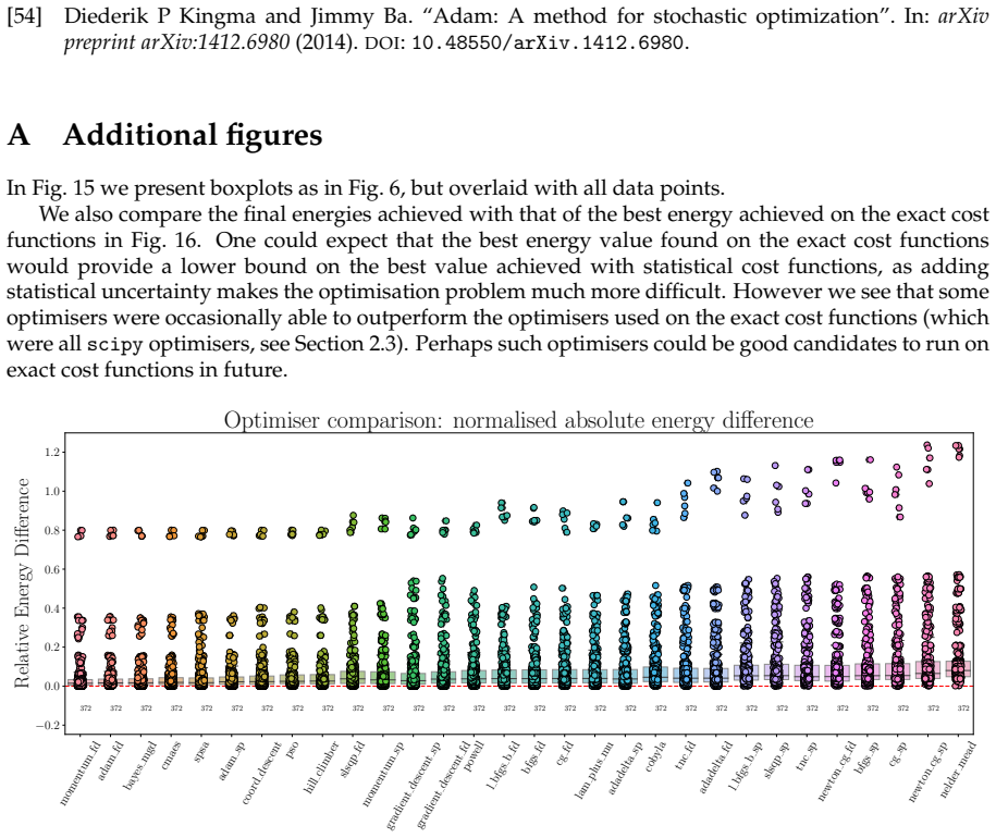
- [Section 2.5 and Fig. 6 caption] The headline ranking compares best-of-multiple-runs for tuned optimisers against a single run for the zero-hyperparameter scipy optimisers. Section 2.5 states that each tuned optimiser is run with at most five sets of hyperparameters (the default plus the best found on each of the four sweeping instances), and the caption of Fig. 6 says that for each optimiser the reported value is 'the best final energy (over different runs, e.g. for multiple hyperparameter settings)'. Since the cost function is stochastic with 1,000 or 10,000 shots, the minimum of five noisy runs is a biased optimistic estimator, whereas COBYLA, Powell, BFGS, L-BFGS-B, TNC, SLSQP, CG, and Newton-CG contribute only a single run per instance. The gaps in Figs. 6, 7, and 9 between the top tuned optimisers and the scipy optimisers could therefore be inflated by the evaluation protocol rather than reflecting genuine optimizer quality. I recommend adding a control that uses only the default hyperparameter set for every optimiser, and/or giving every optimiser the same number of independent restarts, and reporting both the best-of and the median performance.
- [Section 2.4 and Section 2.5] The global finite-difference step size of 0.4 is the average of the best step sizes found on only four instances (0.417, 0.251, 0.324, and 0.550), and the per-optimiser hyperparameters are selected on those same four instances. These sweeping instances are all small (at most 3 × 2 grids and five layers) and do not include the 14-18 qubit or 8-10 layer cases in Benchmarks 3 and 4. Since Fig. 18 shows that optimiser performance varies systematically with U, filling, and number of layers, the representativeness of the four sweeping instances is an unverified assumption that is load-bearing for the claim that '0.4 seemed to be a good choice'. I ask the authors to quantify the sensitivity of the rankings to this choice, for example by re-running the gradient-based optimisers with step sizes near the ends of the observed range (e.g. 0.25 and 0.55) and reporting whether the leading optimisers remain the same.
- [Section 3.2.2 and Fig. 9] For the number-of-calls metric it is not stated whether the reported 'calls to reach tolerance' is taken from the best run over the multiple hyperparameter sets or from each run individually. If Fig. 9 uses the best run for each tuned optimiser and the single run for scipy optimisers, the same best-of-multiple-runs bias applies to the low-call ranking as to the final-energy ranking. The authors should state explicitly how the call counts are aggregated and should report both the best-run and the median-run call counts, so that readers can separate genuine optimizer quality from the number of attempts allowed.
minor comments (4)
- [Table 1] In the row for '3 × 2', the expression '2m⌈ n−1 2 ⌋' mixes a ceiling bracket with a floor symbol; it should read '2m⌈(n−1)/2⌉'.
- [Section 3.2, first paragraph] The phrase 'some plots of individual runs are shown n Fig. 5' should read 'shown in Fig. 5'.
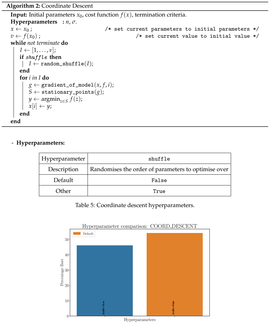
- [Table 15 caption] The caption says 'Coordinate descent hyperparameters', but the table lists Nelder-Mead hyperparameters; the caption should be corrected.
- [Appendix C.4] The word 'Bernouilli' in the SPSA pseudocode description should be spelled 'Bernoulli'.
Circularity Check
No significant circularity: the paper reports directly measured benchmark outcomes, with self-citations only supplying the ansatz and algorithm choices, not the ranking.
full rationale
This is an empirical benchmarking study rather than a derivation, and I find no circular step that makes any reported result equivalent to its inputs by construction. The central claims, such as "Momentum or Adam with finite differences are good optimiser choices when considering overall final accuracy" (Section 4), are summaries of measured final energies over 372 instances, with data hosted on Zenodo. The hyperparameter and gradient sweeping described in Section 2.5 is genuine fitting: the finite-difference step size 0.4 is selected by averaging optimal step sizes on four sweeping instances, and the optimiser rankings are then obtained by running all optimisers on the full instance set. This is parameter selection, not a fitted quantity being renamed as a prediction. Self-citations to the authors' prior work appear, e.g. taking the Hamiltonian variational ansatz and initial parameters "as in [6]" and using BayesMGD from [3], but these citations supply the problem setting and candidate algorithms, not the performance ranking; the rankings are produced by the numerical runs themselves. The paper also openly acknowledges the arbitrariness in hyperparameter choice, stating "There is also much arbitrariness in what one considers a hyperparameter, and one could always promote more variables to hyperparameters and perform more in depth sweeping." The skeptical concern that tuned optimisers receive up to five hyperparameter runs while scipy optimisers receive one is a legitimate evaluation-fairness caveat, and the paper discloses this by taking "the best final energy (over different runs, e.g. for multiple hyperparameter settings)" in Fig. 6; however, this is a possible bias in the benchmark protocol, not a circular dependency in which a claimed prediction reduces to its own input. No equation in the paper defines a target quantity in terms of the fitted hyperparameters, no uniqueness theorem is imported from the authors, and no known result is merely renamed. The derivation chain is therefore self-contained with respect to circularity.
Assumptions & free parameters
free parameters (3)
- Finite-difference step size =
0.4
- Simultaneous perturbation step size =
0.15
- Per-optimizer hyperparameter sets =
varies
assumptions (3)
- domain assumption HV ansatz is expressive enough to approximate the ground states of the tested instances
- domain assumption Shot-noise-only cost function (without physical gate noise) is a valid proxy for near-term hardware
- ad hoc to paper The four instances chosen for hyperparameter sweeping are representative of all 372 instances
Cite this review
Pith. "Pith review of Benchmarking a wide range of optimisers for solving the Fermi-Hubbard model using the variational quantum eigensolver." pith.science (2026). https://pith.science/paper/JOMEX4FO
@misc{pith2026241113742,
  author       = {Pith},
  title        = {Pith review of: Benchmarking a wide range of optimisers for solving the Fermi-Hubbard model using the variational quantum eigensolver},
  year         = {2026},
  howpublished = {\url{https://pith.science/paper/JOMEX4FO}},
  note         = {Machine review of arXiv:2411.13742}
}
read the original abstract
We numerically benchmark 30 optimisers on 372 instances of the variational quantum eigensolver for solving the Fermi-Hubbard system with the Hamiltonian variational ansatz. We rank the optimisers with respect to metrics such as final energy achieved and function calls needed to get within a certain tolerance level, and find that the best performing optimisers are variants of gradient descent such as Momentum and ADAM (using finite difference), SPSA, CMAES, and BayesMGD. We also perform gradient analysis and observe that the step size for finite difference has a very significant impact. We also consider using simultaneous perturbation (inspired by SPSA) as a gradient subroutine: here finite difference can lead to a more precise estimate of the ground state but uses more calls, whereas simultaneous perturbation can converge quicker but may be less precise in the later stages. Finally, we also study the quantum natural gradient algorithm: we implement this method for 1-dimensional Fermi-Hubbard systems, and find that whilst it can reach a lower energy with fewer iterations, this improvement is typically lost when taking total function calls into account. Our method involves performing careful hyperparameter sweeping on 4 instances. We present a variety of analysis and figures, detailed optimiser notes, and discuss future directions.
Figures


Figures from the paper (28 more)






Reference graph
Works this paper leans on
-
[1]
Noisy intermediate-scale quantum algorithms
Kishor Bharti et al. “Noisy intermediate-scale quantum algorithms”. In: Reviews of Modern Physics 94.1 (2022), p. 015004. DOI: 10.1103/RevModPhys.94.015004
-
[2]
Variational quantum algorithms
Marco Cerezo et al. “Variational quantum algorithms”. In: Nature Reviews Physics3.9 (2021), pp. 625–
work page 2021
-
[3]
Stasja Stanisic et al. “Observing ground-state properties of the Fermi-Hubbard model using a scalable algorithm on a quantum computer”. In: Nature Communications 13.1 (2022), p. 5743. DOI: 10.1038/s41467-022-33335-4
-
[4]
Quantum Threat Timeline Report 2022
Michelle Mosca and Marco Piani. Quantum Threat Timeline Report 2022 . Tech. rep. Available at: https://globalriskinstitute.org/publication/2022-quantum-threat-timeline-report/ . EvolutionQ Inc, Global Risk Institute, 2022
work page 2022
-
[5]
Progress towards practical quantum variational algorithms
Dave Wecker, Matthew B Hastings, and Matthias Troyer. “Progress towards practical quantum variational algorithms”. In: Physical Review A 92.4 (2015), p. 042303. DOI: 10.1103/PhysRevA.92. 042303
-
[6]
Strategies for solving the Fermi-Hubbard model on near-term quantum com- puters
Chris Cade et al. “Strategies for solving the Fermi-Hubbard model on near-term quantum com- puters”. In: Physical Review B 102.23 (2020), p. 235122. DOI: 10.1103/PhysRevB.102.235122
-
[7]
Efficient quantum measurement of Pauli operators in the presence of finite sampling error
Ophelia Crawford et al. “Efficient quantum measurement of Pauli operators in the presence of finite sampling error”. In: Quantum 5 (2021), p. 385. DOI: 10.22331/q-2021-01-20-385
-
[8]
Mykel J Kochenderfer and Tim A Wheeler. Algorithms for optimization. MIT Press, 2019. 21
work page 2019
Show all 55 references
-
[9]
Essentials of Metaheuristics
Sean Luke. Essentials of Metaheuristics. second. Available for free at http://cs.gmu.edu/$\sim$sean/book/metaheuristics/. Lulu, 2013
2013
-
[10]
Numerical optimization
Jorge Nocedal and Stephen J Wright. Numerical optimization. Springer, 1999. DOI: 10.1007/978- 0-387-40065-5
1999 doi
- [11]
-
[12]
Sequential minimal optimization for quantum- classical hybrid algorithms
Ken M Nakanishi, Keisuke Fujii, and Synge Todo. “Sequential minimal optimization for quantum- classical hybrid algorithms”. In: Physical Review Research 2.4 (2020), p. 043158. DOI: 10 . 1103 / PhysRevResearch.2.043158
2020
-
[13]
A Jacobi diagonalization and Anderson acceleration algorithm for vari- ational quantum algorithm parameter optimization
Robert M Parrish et al. “A Jacobi diagonalization and Anderson acceleration algorithm for vari- ational quantum algorithm parameter optimization”. In: arXiv preprint arXiv:1904.03206 (2019). DOI: 10.48550/arXiv.1904.03206
-
[14]
Convergence of a block coordinate descent method for nondifferentiable minimiza- tion
Paul Tseng. “Convergence of a block coordinate descent method for nondifferentiable minimiza- tion”. In: Journal of optimization theory and applications 109 (2001), pp. 475–494. DOI: 10.1023/A: 1017501703105
2001 doi
-
[15]
Structure optimization for pa- rameterized quantum circuits
Mateusz Ostaszewski, Edward Grant, and Marcello Benedetti. “Structure optimization for pa- rameterized quantum circuits”. In: Quantum 5 (2021), p. 391. DOI: 10.22331/q-2021-01-28-391
2021 doi
-
[16]
Quantum analytic descent
Bálint Koczor and Simon C Benjamin. “Quantum analytic descent”. In: Physical Review Research 4.2 (2022), p. 023017. DOI: 10.1103/PhysRevResearch.4.023017
2022 doi
-
[17]
Quantum natural gradient
James Stokes et al. “Quantum natural gradient”. In: Quantum 4 (2020), p. 269. DOI: 10.22331/q- 2020-05-25-269
2020 doi
-
[18]
Using models to improve optimizers for variational quantum algorithms
Kevin J Sung et al. “Using models to improve optimizers for variational quantum algorithms”. In: Quantum Science and Technology 5.4 (2020), p. 044008. DOI: 10.1088/2058-9565/abb6d9
2020 doi
-
[19]
Benchmarking a wide range of optimisers for solving the Fermi-Hubbard model using the variational quantum eigensolver
Benjamin D.M. Jones, Lana Mineh, and Ashley Montanaro. Dataset for “Benchmarking a wide range of optimisers for solving the Fermi-Hubbard model using the variational quantum eigensolver” . Hosted at Zenodo, URL: https://doi.org/10.5281/zenodo.13960673. 2024
-
[20]
The variational quantum eigensolver: a review of methods and best practices
Jules Tilly et al. “The variational quantum eigensolver: a review of methods and best practices”. In: Physics Reports 986 (2022), pp. 1–128. DOI: 10.1016/j.physrep.2022.08.003
2022 doi
-
[21]
VQE method: a short survey and recent developments
Dmitry A Fedorov et al. “VQE method: a short survey and recent developments”. In: Materials Theory 6.1 (2022), pp. 1–21. DOI: 10.1186/s41313-021-00032-6
2022 doi
-
[22]
Variational ansatz-based quantum simulation of imaginary time evolution
Sam McArdle et al. “Variational ansatz-based quantum simulation of imaginary time evolution”. In: npj Quantum Information 5.1 (2019), p. 75. DOI: 10.1038/s41534-019-0187-2
2019 doi
-
[23]
Classical optimizers for noisy intermediate-scale quantum devices
Wim Lavrijsen et al. “Classical optimizers for noisy intermediate-scale quantum devices”. In: 2020 IEEE international conference on quantum computing and engineering (QCE). IEEE. 2020, pp. 267–277. DOI: 10.1109/QCE49297.2020.00041
2020
-
[24]
https://scikit-quant.readthedocs.io/en/latest/
Scikit-Quant. https://scikit-quant.readthedocs.io/en/latest/
-
[25]
Performance comparison of optimization methods on variational quantum algorithms
Xavier Bonet-Monroig et al. “Performance comparison of optimization methods on variational quantum algorithms”. In: Physical Review A 107.3 (2023), p. 032407. DOI: 10.1103/PhysRevA.107. 032407
2023 doi
-
[26]
Optimizing quantum heuristics with meta-learning
Max Wilson et al. “Optimizing quantum heuristics with meta-learning”. In: Quantum Machine Intelligence 3 (2021), pp. 1–14. DOI: 10.1007/s42484-020-00022-w
2021 doi
- [27]
-
[28]
Performance of hybrid quantum-classical variational heuristics for combi- natorial optimization
Giacomo Nannicini. “Performance of hybrid quantum-classical variational heuristics for combi- natorial optimization”. In: Physical Review E 99.1 (2019), p. 013304. DOI: 10.1103/PhysRevE.99. 013304
2019 doi
- [29]
-
[30]
Strategies for quantum computing molecular energies using the unitary coupled cluster ansatz
Jonathan Romero et al. “Strategies for quantum computing molecular energies using the unitary coupled cluster ansatz”. In: Quantum Science and Technology 4.1 (2018), p. 014008. DOI: 10.1088/ 2058-9565/aad3e4. 22
2018
-
[31]
Avoiding local minima in varia- tional quantum eigensolvers with the natural gradient optimizer
David Wierichs, Christian Gogolin, and Michael Kastoryano. “Avoiding local minima in varia- tional quantum eigensolvers with the natural gradient optimizer”. In:Physical Review Research 2.4 (2020), p. 043246. DOI: 10.1103/PhysRevResearch.2.043246
2020 doi
- [32]
-
[33]
Classical Benchmarks for Variational Quantum Eigensolver Simula- tions of the Hubbard Model
Antonios M Alvertis et al. “Classical Benchmarks for Variational Quantum Eigensolver Simula- tions of the Hubbard Model”. In: arXiv preprint arXiv:2408.00836 (2024)
2024 arXiv
-
[34]
SciPy 1.0: Fundamental Algorithms for Scientific Computing in Python
Pauli Virtanen et al. “SciPy 1.0: Fundamental Algorithms for Scientific Computing in Python”. In: Nature Methods 17 (2020), pp. 261–272. DOI: 10.1038/s41592-019-0686-2
2020 doi
-
[35]
General parameter-shift rules for quantum gradients
David Wierichs et al. “General parameter-shift rules for quantum gradients”. In: Quantum 6 (2022), p. 677. DOI: 10.22331/q-2022-03-30-677
2022 doi
-
[36]
Estimating the gradient and higher- order derivatives on quantum hardware
Andrea Mari, Thomas R Bromley, and Nathan Killoran. “Estimating the gradient and higher- order derivatives on quantum hardware”. In: Physical Review A 103.1 (2021), p. 012405. DOI: 10. 1103/PhysRevA.103.012405
2021
-
[37]
Optuna: A Next-generation Hyperparameter Optimization Framework
Takuya Akiba et al. “Optuna: A Next-generation Hyperparameter Optimization Framework”. In: Proceedings of the 25th ACM SIGKDD International Conference on Knowledge Discovery and Data Mining. 2019. DOI: 10.1145/3292500.3330701
2019
-
[38]
An overview of the simultaneous perturbation method for efficient optimization
James C Spall. “An overview of the simultaneous perturbation method for efficient optimization”. In: Johns Hopkins apl technical digest 19.4 (1998), pp. 482–492
1998
-
[39]
Implementation of the simultaneous perturbation algorithm for stochastic optimiza- tion
J.C. Spall. “Implementation of the simultaneous perturbation algorithm for stochastic optimiza- tion”. In: IEEE Transactions on Aerospace and Electronic Systems 34.3 (1998), pp. 817–823. DOI: 10. 1109/7.705889
1998
-
[40]
DEAP: Evolutionary Algorithms Made Easy
Félix-Antoine Fortin et al. “DEAP: Evolutionary Algorithms Made Easy”. In: Journal of Machine Learning Research 13 (2012), pp. 2171–2175
2012
-
[41]
Completely derandomized self-adaptation in evolu- tion strategies
Nikolaus Hansen and Andreas Ostermeier. “Completely derandomized self-adaptation in evolu- tion strategies”. In:Evolutionary computation 9.2 (2001), pp. 159–195.DOI: 10.1162/106365601750190398
2001 doi
- [42]
-
[43]
Implementing the Nelder-Mead simplex algorithm with adaptive parameters
Fuchang Gao and Lixing Han. “Implementing the Nelder-Mead simplex algorithm with adaptive parameters”. In: Computational Optimization and Applications 51.1 (2012), pp. 259–277. DOI: 10 . 1007/s10589-010-9329-3
2012
-
[44]
A simplex method for function minimization
John A Nelder and Roger Mead. “A simplex method for function minimization”. In: The computer journal 7.4 (1965), pp. 308–313. DOI: 10.1093/comjnl/7.4.308
1965 doi
-
[45]
A direct search optimization method that models the objective and constraint func- tions by linear interpolation
Michael JD Powell. A direct search optimization method that models the objective and constraint func- tions by linear interpolation. Springer, 1994. DOI: 10.1007/978-94-015-8330-5_4
1994 doi
-
[46]
A view of algorithms for optimization without derivatives
Michael JD Powell. “A view of algorithms for optimization without derivatives”. In: Mathematics Today-Bulletin of the Institute of Mathematics and its Applications 43.5 (2007), pp. 170–174
2007
- [47]
-
[48]
Natural gradient works efficiently in learning
Shun-Ichi Amari. “Natural gradient works efficiently in learning”. In: Neural computation 10.2 (1998), pp. 251–276. DOI: 10.1162/089976698300017746
1998 doi
- [49]
-
[50]
Low-depth gradient measurements can improve conver- gence in variational hybrid quantum-classical algorithms
Aram W Harrow and John C Napp. “Low-depth gradient measurements can improve conver- gence in variational hybrid quantum-classical algorithms”. In:Physical Review Letters126.14 (2021), p. 140502. DOI: 10.1103/PhysRevLett.126.140502
2021 doi
-
[51]
On the momentum term in gradient descent learning algorithms
Ning Qian. “On the momentum term in gradient descent learning algorithms”. In: Neural networks 12.1 (1999), pp. 145–151. DOI: 10.1016/S0893-6080(98)00116-6
1999 doi
- [52]
-
[53]
Adaptive subgradient methods for online learning and stochastic optimization
John Duchi, Elad Hazan, and Yoram Singer. “Adaptive subgradient methods for online learning and stochastic optimization”. In: Journal of machine learning research 12.7 (2011). 23
2011
-
[54]
Adam: A method for stochastic optimization
Diederik P Kingma and Jimmy Ba. “Adam: A method for stochastic optimization”. In: arXiv preprint arXiv:1412.6980 (2014). DOI: 10.48550/arXiv.1412.6980. A Additional figures In Fig. 15 we present boxplots as in Fig. 6, but overlaid with all data points. We also compare the fina...
-
[644]
DOI: 10.1038/s42254-021-00348-9
Reviewed August 12, 2026 · model on record in the stance chip above.
Discussion (0). Continue with ORCID to comment.