REVIEW 2 major objections 3 minor 13 references
Generative AI for Music and Audio
T0 review · 2 major / 3 minor · reviewed 2026-08-12 · deepseek-v4-flash
Pith's one-line read Text-queried sound separation and text-to-audio synthesis can be learned from unlabeled video alone, with CLIP's image-text embedding space serving as the bridge from text to audio.
desk verdict This is a thesis-by-publications, not a new research paper: no new technical claims, but the constituent papers are solid, and the only real overstatement is the word 'universal' in the CLIPSep chapter, which the author's own ESC-50 results undercut. read the letter →
The pith
A machine-rendered reading of the paper's core claim, the machinery that carries it, and where it could break.
The reading
What carries the argument
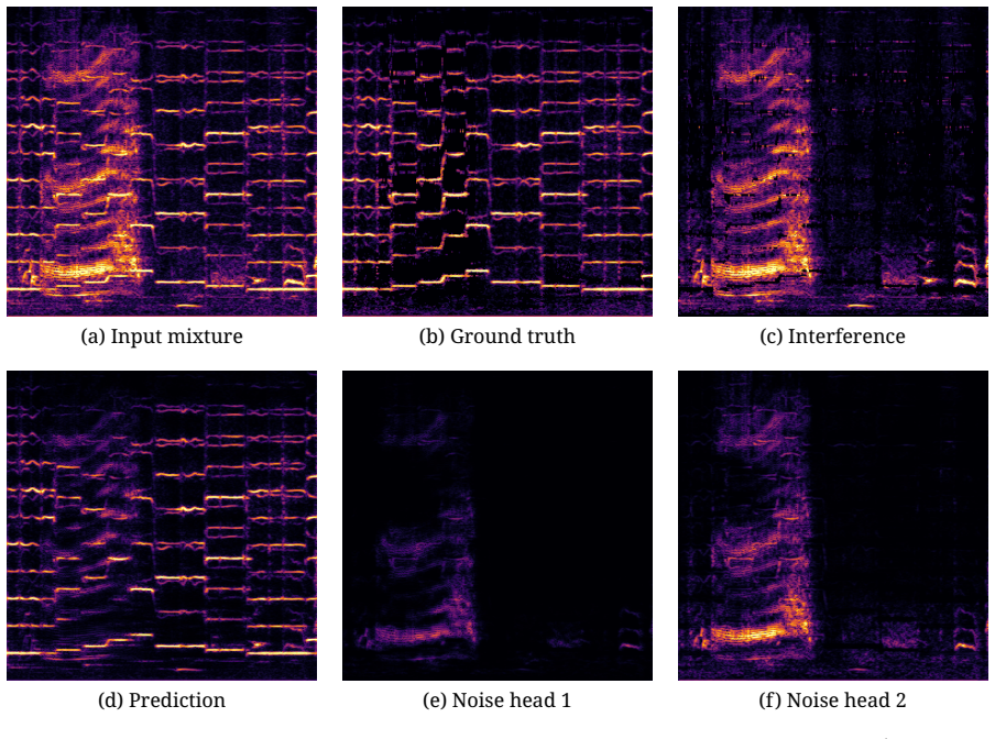
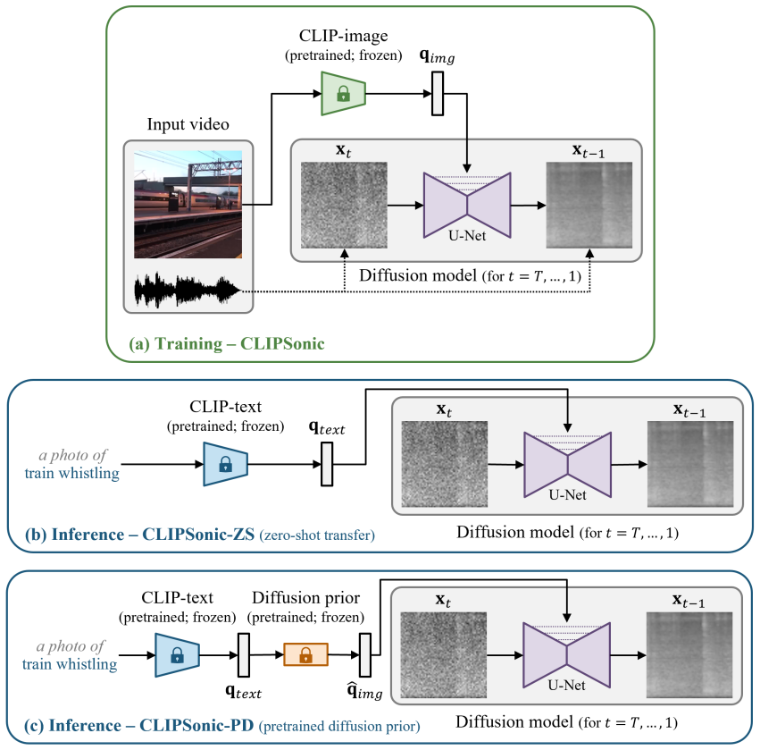
The load-bearing mechanism is the frozen CLIP embedding space, a pretrained joint representation in which matching images and texts are close together, used as a fixed bridge between text, image, and, through video, audio. During training a video frame is encoded by CLIP's image encoder and projected into a query vector that mixes an over-determined set of masks produced by an audio U-Net; at test time a text prompt is encoded by CLIP's text encoder and fed down the same path. The second mechanism, noise invariant training, adds permutation-invariant noise heads whose outputs are interchangeable in the loss so that off-screen and background sounds are absorbed during training and discarded at inference.
What would settle it
Evaluate a CLIPSep-NIT model trained on unlabeled VGGSound video on mixtures whose target sounds are textually clear but visually unobservable, such as a dog barking off-screen or an obscured alarm clock: if text-queried SDR is no better than the input mixture while a supervised text-queried model succeeds, the claimed zero-shot visual bridge is refuted.
Extended reading notes
Core claim
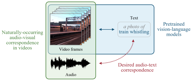
The central discovery is that the visual modality can supply the semantic supervision that text-audio pairs normally provide. CLIPSep trains an audio separation model on image-audio pairs cropped from video: the CLIP image encoder turns a video frame into a query vector, that query vector weights a bank of intermediate masks from an audio U-Net, and the model is trained to separate the audio that corresponds to the image. At test time the same pathway is fed a text embedding from CLIP, and because CLIP was trained to put matching images and text close together, the text query separates the target sound without any text-audio training data. Because real videos contain off-screen sounds and background noise, CLIPSep-NIT adds permutation-invariant noise heads that absorb query-irrelevant audio during training and are discarded at inference. The reported numbers show text-queried separation learned from unlabeled video reaching competitive performance against a supervised model in some settings, and CLIPSonic carries the same bridge over to text-to-audio synthesis.
Load-bearing premise
The load-bearing premise is that CLIP's shared text-image embedding space lines up with audio content well enough that a text prompt can replace the video-frame query the model was trained on.
Editorial extensions
If this is right
- Text-queried universal sound separation can be trained without labeled text-audio data, using only the naturally occurring audio-visual correspondence in unlabeled video.
- On the MUSIC+ evaluation the label-free CLIPSep-NIT model lands within 0.46 dB mean SDR of a fully supervised text-queried model and edges ahead on median SDR.
- The same bridge is reusable for text-to-audio synthesis, so a single idea covers both separation and generation with no text-audio pairs.
- Because noise heads absorb irrelevant sound during training, the approach tolerates the off-screen audio and background noise that dominate internet video.
- Text, image, and hybrid queries share one query pathway, and multiple queries can be combined to extract several target sounds from one mixture.
Reading between the lines
- If the bridge holds, the practical ceiling for such systems is set by CLIP's text-image alignment rather than by available audio labels, so improving or specializing the joint embedding space should directly improve separation quality.
- The reported modality-transfer gaps of 0.88 to 1.79 dB SDR measure exactly the cost of replacing an image query with a text query; a testable prediction is that fine-tuning the CLIP encoders on target-domain audio-visual data would shrink those gaps.
- The video-bridge strategy should falter for sounds whose visual and acoustic identities diverge, such as off-screen or invisible sources, so the approach is best understood as a method for visually grounded sound classes.
- The same noise-invariant conditioning principle could be carried into adjacent generation tasks, such as text-conditioned music generation or video-to-audio synthesis, where unlabeled video is abundant and paired supervision is scarce.
Editorial analysis
A structured set of objections, weighed in public.
Referee Report
Summary. This dissertation compiles six previously published papers by the author into three research directions: multitrack music generation (MusPy and MMT), assistive music creation tools (automatic instrumentation and Deep Performer), and multimodal learning for audio and music (CLIPSep and CLIPSonic). The central technical contribution, carried by Chapter 6, is CLIPSep, a text-queried sound separation model trained without labeled audio-text pairs by using CLIP image-text embeddings together with noisy unlabeled videos, and its extension CLIPSep-NIT with noise-invariant training. Chapter 7 applies the same video-bridged idea to CLIPSonic for text-to-audio synthesis. Each chapter reports experiments, ablations, subjective tests, and, for several components, releases code repositories.
Significance. If the central claim holds, the dissertation demonstrates a scalable route to text-audio alignment for separation and synthesis without paired text-audio supervision, using only unlabeled video and a frozen CLIP model; this could substantially reduce data collection cost for controllable audio tools. The work has notable strengths: the MusPy, MMT, and CLIPSep repositories are linked, hyperparameters are reported in detail, systematic ablations are provided (e.g., feature and augmentation ablations in Chapter 4, positional-encoding ablations in Chapter 5, noise-regularization sweeps in Chapter 6), and the self-attention analysis in Chapter 3 is a useful contribution. However, the 'universal' label attached to the Chapter 6 results is broader than the evidence supports, because the zero-shot modality transfer is demonstrated mainly on visually salient classes and fails on ESC-50 without finetuning.
major comments (2)
- [Chapter 6 abstract; Table 6.6; Section 6.5] The abstract's claim that CLIPSep successfully learns 'text-queried universal sound separation' is not supported for non-visually-salient or ambient sound classes. In the zero-shot transfer experiment of Section 6.H/Table 6.6, the CLIPSep model trained on VGGSound achieves a mean SDR of 1.07 dB on ESC-50 against a 0.00 dB mixture baseline, which is effectively no separation, whereas finetuning on ESC-50 raises the mean SDR to 6.73 dB. The paper does not report an ESC-50 result for CLIPSep-NIT, so the best unlabeled variant's universality remains untested. Since Section 6.5 itself concedes that the approach 'requires a sufficient audio-visual correspondence,' the qualifier 'universal' should be replaced or explicitly scoped to visually salient classes, or supported by evidence on diverse non-visual and ambient sound categories.
- [Section 5.3 and Section 5.4] The Deep Performer results are not fully reproducible because the inversion model is trained on an internal 156-hour commercial recording dataset that is not released. The final audio quality reported in the subjective listening test (Table 5.2) comes from the complete three-stage pipeline, so the unreleased inversion training data is a load-bearing component of the Chapter 5 comparison. I ask the authors to release the dataset or a suitable substitute, provide a released pretrained inversion checkpoint with its provenance, or clearly state this dependency as a reproducibility limitation.
minor comments (3)
- [Section 3.4.2, Table 3.2] The subjective listening test in Chapter 3 uses only 9 participants recruited from the authors' social networks, and the overall MOS confidence intervals overlap substantially (MMT 3.33±0.47, REMI+ 3.77±0.41); the 'comparable performance' wording should be tempered or supplemented with a significance test.
- [Sections 1.3, 6.1, and 7.1] Several passages assert 'the first' model for a given task without a systematic prior-art search; these priority claims should be softened to 'to our knowledge' or supported by a dedicated related-work survey.
- [Sections 3.3.1, 4.3, 6.1, and 6.4.3] There are minor typos and grammatical errors, including 'propsoed' (Section 3.3.1), 'assisstive' (Section 4.3), 'an our demo website' (Section 6.1), and 'we mix the an audio sample' (Section 6.4.3); these should be corrected before publication.
Circularity Check
No significant circularity: the dissertation's core claims are empirically evaluated against external baselines and its acknowledged limitations are not circular reductions.
full rationale
No circularity found. The load-bearing technical claim in Chapter 6 is that CLIPSep learns text-queried separation from unlabeled videos by using the pretrained CLIP image-text embedding as a bridge between audio and text. The defining equations (6.1) and (6.2)-(6.6) train image-conditioned mask predictors with self-supervised mixture losses; the text query at test time is encoded by the frozen external CLIP model, whose stated assumptions do not include the separation result, so no prediction reduces to the paper's own fitted parameters by construction. Text-query SDRs in Tables 6.2 and 6.3 are measured on held-out mixtures and compared against supervised baselines such as LabelSep, BERTSep, and CLIPSep-Text. The paper also explicitly acknowledges the modality-transfer gap and its cause in Section 6.5 ('it still requires a sufficient audio-visual correspondence for training video'), and Appendix 6.H reports a negative zero-shot ESC-50 result (mean SDR 1.07 dB vs 0.00 dB for the mixture), which is an honest limitation statement rather than a circular step. Chapters 2-5 are reprints of the author's prior publications with external comparisons (e.g., MMM, REMI+, Hifi-GAN); the self-citations scattered through the introduction are provenance statements, not load-bearing mathematical premises. There is no self-authored uniqueness theorem invoked to force a choice, and no fitted parameter is renamed as a prediction. The absence of a CLIPSep-NIT ESC-50 result is a missing-evidence concern for the 'universal' claim, but it does not make any derivation equivalent to its inputs.
Assumptions & free parameters
free parameters (3)
- Noise regularization level gamma (CLIPSep-NIT) =
0.25
- Noise regularization weight lambda (CLIPSep-NIT) =
0.1
- Top-k sampling fraction per field (MMT) =
10% of possible outcomes per field
assumptions (3)
- domain assumption The pretrained CLIP text-image embedding space transfers to audio at test time (zero-shot modality transfer).
- domain assumption DTW alignments between synthesized scores and recordings provide sufficient supervision for the alignment model.
- domain assumption Small listener panels from the authors' social networks represent target users.
Cite this review
Pith. "Pith review of Generative AI for Music and Audio." pith.science (2026). https://pith.science/paper/XQK3XJKJ
@misc{pith2026241114627,
  author       = {Pith},
  title        = {Pith review of: Generative AI for Music and Audio},
  year         = {2026},
  howpublished = {\url{https://pith.science/paper/XQK3XJKJ}},
  note         = {Machine review of arXiv:2411.14627}
}
read the original abstract
Generative AI has been transforming the way we interact with technology and consume content. In the next decade, AI technology will reshape how we create audio content in various media, including music, theater, films, games, podcasts, and short videos. In this dissertation, I introduce the three main directions of my research centered around generative AI for music and audio: 1) multitrack music generation, 2) assistive music creation tools, and 3) multimodal learning for audio and music. Through my research, I aim to answer the following two fundamental questions: 1) How can AI help professionals or amateurs create music and audio content? 2) Can AI learn to create music in a way similar to how humans learn music? My long-term goal is to lower the barrier of entry for music composition and democratize audio content creation
Figures


Figures from the paper (52 more)












Reference graph
Works this paper leans on
-
[1]
TensorFlow: A system for large- scale machine learning
Warden, Martin Wicke, Yuan Yu, and Xiaoqiang Zheng (2016). “TensorFlow: A system for large- scale machine learning.” USENIX Symposium on Operating Systems Design and Implementation (OSDI) (cited on pages 9, 12, 42). Yuzo Abe, Yuki Murakami, and Masanobu Miura (2012). “Automatic arrangement for the bass guitar in popular music using principle component ana...
work page 2016
-
[2]
MusicLM: Generating Music From Text
Huang, Aren Jansen, Adam Roberts, Marco Tagliasacchi, Matt Sharifi, Neil Zeghidour , and Chris- tian Frank (2023). “MusicLM: Generating Music From Text.” arXiv preprint arXiv:2302.03917 (cited on pages 94, 95). Relja Arandjelović and Andrew Zisserman (2017a). “Look, listen and learn.” International Conference on Computer Vision (ICCV) (cited on page 79). ...
arXiv 2023
-
[3]
Language Models are Few-Shot Learners
Chess, Jack Clark, Christopher Berner, Sam McCandlish, Alec Radford, Ilya Sutskever, and Dario Amodei (2020). “Language Models are Few-Shot Learners.” Advances in Neural Information Processing Systems (NeurIPS) (cited on pages 27, 75). Emilios Cambouropoulos (2006). “‘Voice’ separation: theoretical, perceptual and computational per- spectives.” Internatio...
arXiv 2020
-
[4]
CLIPSynth: Learning Text-to-audio Synthesis from Videos using CLIP and Diffusion Models
Chen, Arpit Gupta, Tagyoung Chung, Jing Huang, Nanyun Peng, and Wenbo Zhao (2023c). “CLIPSynth: Learning Text-to-audio Synthesis from Videos using CLIP and Diffusion Models.” CVPR Workshop on Sight and Sound (WSS) (cited on pages 2, 5, 95). 115 Hao-Wen Dong, Naoya Takahashi, Yuki Mitsufuji, Julian McAuley, and Taylor Berg-Kirkpatrick (2023d). “CLIPSep: Le...
arXiv 2023
-
[5]
AudioGen: Textually Guided Audio Generation
Parikh, Yaniv Taigman, and Yossi Adi (2023). “AudioGen: Textually Guided Audio Generation.” International Conference on Learning Representations (ICLR) (cited on page 94). Kundan Kumar, Rithesh Kumar, Thibault de Boissiere, Lucas Gestin, Wei Zhen Teoh, Jose Sotelo, Alexandre de Brebisson, Yoshua Bengio, and Aaron Courville (2019). “MelGAN: Generative Adve...
work page 2023
-
[6]
WavJourney: Compositional Audio Creation with Large Language Models
Kong, Mark D. Plumbley, and Wenwu Wang (2023b). “WavJourney: Compositional Audio Creation with Large Language Models.” arXiv preprint arXiv:2307.14335 (cited on page 109). Magenta (n.d.). url: https://magenta.tensorflow.org/ (cited on page 9). Rachel Manzelli, Vijay Thakkar, Ali Siahkamari, and Brian Kulis (2018). “Conditioning Deep Generative Raw Audio M...
arXiv 2023
-
[7]
PyTorch: An Imperative Style, High-Performance Deep Learning Library
Fang, Junjie Bai, and Soumith Chintala (2019). “PyTorch: An Imperative Style, High-Performance Deep Learning Library.” Advances in Neural Information Processing Systems (NeurIPS) (cited on pages 12, 82). Christine Payne (2019).MuseNet. OpenAI Blog. url: https://openai.com/blog/musenet/ (cited on pages 23, 24, 37). Karol J. Piczak (2015). “ESC: Dataset for...
work page 2019
-
[8]
Learning Transferable Visual Models From Natural Language Supervision
Sastry, Amanda Askell, Pamela Mishkin, Jack Clark, Gretchen Krueger, and Ilya Sutskever (2021). “Learning Transferable Visual Models From Natural Language Supervision.” International Conference on Machine Learning (ICML) (cited on pages 65, 68, 69, 81, 94). Alec Radford, Jeff Wu, Rewon Child, David Luan, Dario Amodei, and Ilya Sutskever (2019). “Language ...
arXiv 2021
Show all 13 references
-
[9]
DeepSinger: Singing Voice Synthesis with Data Mined From the Web
Fast, Robust and Controllable Text to Speech.” Advances in Neural Information Processing Systems (NeurIPS) (cited on pages 52, 55, 62). Yi Ren, Xu Tan, Tao Qin, Jian Luan, Zhou Zhao, and Tie-Yan Liu (2020). “DeepSinger: Singing Voice Synthesis with Data Mined From the Web.”Con...
2020
-
[10]
AVLnet: Learning Audio-Visual Language Representations from Instructional Videos
Picheny, Antonio Torralba, and James Glass (2021). “AVLnet: Learning Audio-Visual Language Representations from Instructional Videos.” Annual Conference of the International Speech Communication Association (INTERSPEECH) (cited on page 103). Andrew Rouditchenko, Hang Zhao, Chu...
2021 arXiv
-
[11]
LAION-5B: An open large-scale dataset for training next generation image-text models
Cherti, Theo Coombes, Aarush Katta, Clayton Mullis, Mitchell Wortsman, Patrick Schramowski, Srivatsa Kundurthy, Katherine Crowson, Ludwig Schmidt, Robert Kaczmarczyk, and Jenia Jitsev (2022). “LAION-5B: An open large-scale dataset for training next generation image-text models...
2022
-
[12]
Natural TTS Synthesis by Conditioning WaveNet on Mel Spectrogram Predictions
Chen, Yu Zhang, Yuxuan Wang, RJ Skerry-Ryan, Rif A. Saurous, Yannis Agiomyrgiannakis, and Yonghui Wu (2018). “Natural TTS Synthesis by Conditioning WaveNet on Mel Spectrogram Predictions.” IEEE International Conference on Acoustics, Speech, and Signal Processing (ICASSP) (cite...
2018 arXiv
-
[13]
Tacotron: Towards End-to-End Speech Synthesis
Yang, Ying Xiao, Zhifeng Chen, Samy Bengio, Quoc Le, Yannis Agiomyrgiannakis, Rob Clark, and Rif A. Saurous (2017). “Tacotron: Towards End-to-End Speech Synthesis.” Annual Conference of the International Speech Communication Association (INTERSPEECH) (cited on page 51). Ziyu W...
2017 arXiv
Reviewed August 12, 2026 · model on record in the stance chip above.
Discussion (0). Continue with ORCID to comment.