REVIEW 3 major objections 4 minor 63 references
HotSpot: Signed Distance Function Optimization with an Asymptotically Sufficient Condition
T0 review · 3 major / 4 minor · reviewed 2026-08-12 · deepseek-v4-flash
Pith's one-line read A heat-diffusion loss provably drives neural signed distances to the true distance function.
desk verdict Strong empirical paper with a real proof gap: Eq. (38) bounds distance to the artificial ε-balls, not to the interpolated surface, so the headline 'asymptotically sufficient condition' is not established as stated. read the letter →
The pith
A machine-rendered reading of the paper's core claim, the machinery that carries it, and where it could break.
The reading
What carries the argument
The machinery is the screened Poisson equation $\nabla^2 h - \lambda^2 h = 0$ with the Dirichlet condition $h = 1$ on the target surface, together with the classical heat–distance relation $\lim_{\lambda\to\infty} \frac{1}{\lambda}\ln h_\lambda(x) = -d_\Gamma(x)$, which says the log of an absorbed heat field recovers the distance to the boundary as absorption grows. The paper turns this PDE into a trainable loss by substituting $h(x) = e^{-\lambda|u(x)|}$ into the energy functional $\frac{1}{2}\int_\Omega \|\nabla h\|^2 + \lambda^2 h^2\,dx$, yielding the heat loss whose variation recovers the screened Poisson equation. The absorption coefficient $\lambda$ is the accuracy knob: the supplement proves the recovered field $|u_\lambda| = -\frac{1}{\lambda}\ln h_\lambda$ deviates from $d_\Gamma$ by $1/\lambda$-order terms that depend on $\ln(\varepsilon/d_\Gamma)$ and $\ln N$, where $N$ is the number of input points.
What would settle it
Solve the screened Poisson equation numerically for a known analytic surface with $h = 1$ on a densely sampled boundary, recover $u_\lambda = -\frac{1}{\lambda}\ln h_\lambda$, and check whether $d_\Gamma(x) - |u_\lambda(x)|$ stays within the paper's bound and falls linearly with $1/\lambda$ as $\lambda$ grows. Then thin the samples until the proof's assumption that boundary balls do not influence each other clearly fails, and test whether the minimizer of the heat loss still converges to a true signed distance; if the error leaves the predicted envelope, or remains distant at those densities, the asymptotic sufficiency claim is limited to the dense regime.
Extended reading notes
Core claim
The central claim is that minimizing the heat loss $L_{\mathrm{heat}} = \frac{1}{2}\int_\Omega e^{-2\lambda|u(x)|}\left(\|\nabla u(x)\|^2 + 1\right)\,dx$, together with a boundary term that pins $u$ to zero at the input points, makes the recovered field converge to the true signed distance as $\lambda \to \infty$. The paper proves that the solution of the screened Poisson equation $\nabla^2 h - \lambda^2 h = 0$, with $h = e^{-\lambda\varepsilon}$ on small balls of radius $\varepsilon$ around the sample points, satisfies $\frac{1}{\lambda}\ln\frac{\varepsilon}{d_\Gamma(x)} \le d_\Gamma(x) - |u_\lambda(x)| \le \frac{1}{\lambda}\left(\ln\frac{\varepsilon}{d_\Gamma(x)} + \ln N\right)$, so the error is first-order small in $1/\lambda$. Because the heat loss is the variational form of that equation under the substitution $h = e^{-\lambda|u|}$, its minimizer inherits this heat–distance behavior, in contrast to eikonal-type losses that are only necessary conditions and admit non-distance solutions even when minimized almost everywhere. Three structural consequences follow: spatial stability (a perturbation of the field decays exponentially instead of traveling along rays), temporal stability (the gradient flow is the heat equation and converges), and an automatic penalty on large surfaces through a coarea-type bound that does not distort the level sets.
Load-bearing premise
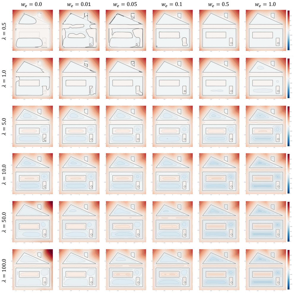
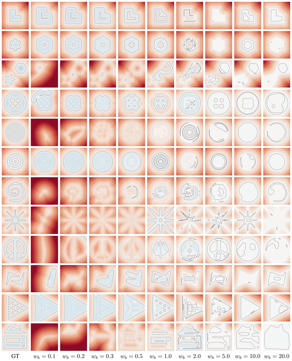
The proof assumes the input points are dense enough that a continuous surface connecting them can act as a firm boundary where the heat field is held at a constant value, whereas the optimizer enforces that boundary only softly with a weighted loss; if the points are too sparse or the boundary weight too small, the signed distance can collapse into an unsigned one.
Editorial extensions
If this is right
- Raw point clouds yield better surfaces: on ShapeNet the method reports IoU 0.9796 against 0.9641 for the strongest compared baseline, with lower Chamfer and Hausdorff distances, and on high-genus shapes it recovers the correct topology where baselines produce extra boundaries.
- Distance queries become more reliable exactly where they matter: near-surface errors drop by more than a third relative to the best baseline on the paper's ShapeNet metrics, and sphere tracing converges in fewer steps as a direct result.
- Optimization is provably better behaved: the heat-loss gradient flow is the heat equation and converges, while a local perturbation of the field decays exponentially instead of persisting along characteristic lines as it does for the eikonal equation.
- Area shrinkage no longer distorts the field: because the heat loss upper-bounds a coarea term, large surfaces are penalized automatically, and the separate area regularizers that bend the level sets of prior methods become unnecessary.
- Accuracy is predictable in advance: the linear-in-$1/\lambda$ bound means the residual error of a trained field is controlled by $\lambda$, the sampling scale $\varepsilon$, and the point count $N$, which the paper exploits through a $\lambda$ scheduler.
Reading between the lines
- The bound suggests a density-aware default for $\lambda$ that the paper leaves implicit: with an estimate of the point spacing and a target error tolerance, Eq. 38 can be inverted to choose $\lambda$ up front, turning the hand-tuned scheduler into a parameter-free recipe.
- A testable prediction of the theory is a sharp phase transition in point-cloud density: reconstruction quality should degrade abruptly once the mean spacing approaches the scale of the boundary balls used in the proof, and the error bound should visibly break at that density.
- Because the loss needs only the field value and its first derivative, and the boundary condition is the only geometric input, the same construction could attach the screened-Poisson boundary to silhouettes or depth maps rather than points, which would extend the asymptotically sufficient guarantee to image-driven reconstruction; the paper lists inverse rendering as future work without making this
- The stability analysis applies just as well to initialization noise as to injected errors, so the heat loss should make results less sensitive to random seeds than eikonal training, a comparison the paper does not run.
Editorial analysis
A structured set of objections, weighed in public.
Referee Report
Summary. The paper proposes HotSpot, a loss for optimizing neural signed distance functions based on the screened Poisson equation. The authors derive a heat loss L_heat = (1/2)∫ e^{-2λ|u|}(||∇u||² + 1) dx, whose minimizer in the heat-field variable satisfies the screened Poisson equation, and they prove a bound (Eq. 9 / Eq. 38 in the supplement) showing that the recovered distance |u_λ| converges linearly to the true distance as λ→∞. The paper also claims spatial and temporal stability, natural surface-area penalization, and a connection to the PHASE method. Experiments on 2D and 3D datasets, including ShapeNet and high-genus shapes, report improved reconstruction and distance metrics over baselines such as DiGS and StEik.
Significance. If the theoretical claim holds, this is a valuable contribution to neural SDF optimization: it offers a principled alternative to the eikonal loss with a quantitative convergence guarantee, grounded in Varadhan's classical heat-kernel asymptotics. The paper is well-written, the derivations are mostly transparent, and the empirical gains are substantial and consistently presented across multiple datasets and metrics. The authors also honestly discuss the fragility of the boundary condition and disclose the relationship to PHASE. However, the central theoretical claim rests on a proof that currently has a concrete mathematical flaw and a gap between the discrete boundary used in the proof and the continuous surface claimed in the main text.
major comments (3)
- [Section 3 and Supplement A.3, Eqs. (30)-(38)] The bound in Eq. (9)/(38) is proven for a discrete boundary consisting of balls B(x_i, ε) around the input points, not for the continuous interpolated surface Γ. The proof explicitly assumes the isolation condition h_j(S_i)=h_j(x_i) for i≠j and ε<r_0, which only holds when the balls are well separated and inter-ball influence is negligible. The main text asserts that 'if there are some boundaries connecting them, the boundary condition of Eq. (4) still holds' (Section 3), but this is not proved. Consequently, the central claim that |u_λ| converges to d_Γ (the distance to the interpolated surface) is not established; at best the proof controls the distance to the point cloud with artificial balls, which differs from d_Γ by a non-vanishing amount in the limit λ→∞. This gap needs to be closed, or the claim should be reformulated to state what is actually proven.
- [Supplement A.3, Eq. (37)] The lower-bound proof contains an incorrect inequality. The function h0(r)=ε/r e^{-λr} is positive and decreasing for r≥ε. Since Σc_i r_i/Σc_i ≥ d_Γ(x), the second inequality in Eq. (37) should read h0(Σc_i r_i/Σc_i) ≤ h0(d_Γ(x)), not ≥. As written, the chain does not imply h(x) ≥ ε e^{-λd_Γ}/d_Γ. The lower bound in Eq. (38) is therefore not proven by the given argument. The upper bound appears correct, but the lower bound is essential for the claimed two-sided convergence rate.
- [Section 4.2.2, Eqs. (14)-(15)] The temporal stability analysis is performed for the gradient flow in the heat-field variable h, ∂h/∂t = ∇²h - λ²h. However, the actual optimization is on the network output u with the combined loss of Eq. (8). The dynamics of u under gradient descent are not governed by this h-heat equation, and the assertion that |u| converges because the h-flow is stable and 'u is continuous' is not justified. The temporal stability claim for the proposed method is therefore unsupported as stated.
minor comments (4)
- [Section 4.3, Eq. (17)] The claimed Euler-Lagrange equation for the coarea loss is incorrect. A direct computation gives ∇·(e^{-λ|u|}∇u/||∇u||) + λ sgn(u)e^{-λ|u|}||∇u|| = 0, which for ||∇u||=1 reduces to a mean-curvature condition, not 1-∇²u=0. This does not invalidate the qualitative conclusion, but the stated derivation should be corrected or removed.
- [Section 4.1, around Eq. (8)] The phrase 'our loss, when minimized, provides an asymptotically sufficient condition' should be qualified: the theoretical claim concerns the exact minimizer of the heat-loss energy functional, whereas the method minimizes a weighted combination of boundary, eikonal, and heat losses with a neural network. A brief discussion of the approximation gap would avoid overclaiming.
- [Section 5.3] The λ scheduler used in the ShapeNet experiments is described in the supplement but not in the main text; a short description in the main text would improve reproducibility.
- [Section 4.2.1 and Supplement C] There are minor typos: 'presist' in the paragraph before Proposition 1 and 'backproping' in Supplement C.
Circularity Check
No significant circularity: the asymptotic sufficiency bound is derived from an external PDE limit theorem with explicit non-fitted constants, and the disclosed PHASE equivalence is a novelty caveat, not a circular reduction.
full rationale
Walking the derivation chain: the heat loss is constructed by substituting h=e^{-\lambda |u|} into a screened-Poisson energy whose Euler-Lagrange equation is \nabla^2 h - \lambda^2 h = 0, and the claimed convergence to a distance function rests on Varadhan's classical limit (Eq. 5, ref [6]), an external and parameter-free theorem. The supplement A.3 bound (Eq. 38) is proved directly on the explicit PDE solution h = \epsilon \sum c_i e^{-\lambda r_i}/r_i with explicit constants \epsilon, N, and d_\Gamma(x); no data are fitted and then reinterpreted as a prediction. The paper openly discloses that its regularizer is closely related to Lipman's PHASE energy under the change h = 1 - |o| (Supp. C), so the PHASE connection affects novelty rather than constituting a hidden reuse of the paper's own conclusions. The reviewer-identified weakness is a genuine unproven assumption: the passage from d_\Gamma for the interpolated surface \Gamma to the artificial ball-boundary set \cup_i B(x_i,\epsilon) relies on the assertion in Section 3 that 'if there are some boundaries connecting them, the boundary condition of Eq. (4) still holds' and on the isolation assumption h_j(S_i)=h_j(x_i) in A.3. Moreover, the implemented objective enforces the boundary only softly through w_b and depends on spectral-bias interpolation, so the theoretical guarantee is not fully realized by the finite-weight loss. These are correctness and assumption gaps, not circular reductions: Eq. (38) does not reduce to any fitted input, and the sufficiency claim is not identical to the loss definition by construction. The only self-citation involving an author (ref [41], a differentiable-rendering paper) appears in a survey list and is not load-bearing. Accordingly, no circular step is exhibited.
Assumptions & free parameters
free parameters (3)
- absorption coefficient λ =
scheduled in training, exact values not in text
- boundary ball radius ε in the proof =
not specified (analysis parameter)
- loss weights w_b, w_e, w_h =
not reported in visible text
assumptions (5)
- standard math Varadhan's heat-kernel limit: for the solution h_λ of the screened Poisson equation (Eq. 4), lim_{λ→∞} (1/λ) ln h_λ(x) = -d_Γ(x)
- domain assumption The input point cloud can be replaced by a continuous surface superset Γ interpolating the points, so the Dirichlet boundary condition h = 1 holds on Γ
- ad hoc to paper Isolation assumption in the discrete proof: for i≠j, h_j(S_i) = h_j(x_i), and the ball radius ε satisfies ε < r_0
- domain assumption Neural networks interpolate between boundary points via spectral bias, so the soft boundary loss effectively enforces the boundary on the interpolated surface
- domain assumption The function-space minimizer of the loss and the h-space gradient flow represent the trained network's behavior
Cite this review
Pith. "Pith review of HotSpot: Signed Distance Function Optimization with an Asymptotically Sufficient Condition." pith.science (2026). https://pith.science/paper/NQNJSXMS
@misc{pith2026241114628,
  author       = {Pith},
  title        = {Pith review of: HotSpot: Signed Distance Function Optimization with an Asymptotically Sufficient Condition},
  year         = {2026},
  howpublished = {\url{https://pith.science/paper/NQNJSXMS}},
  note         = {Machine review of arXiv:2411.14628}
}
read the original abstract
We propose a method, HotSpot, for optimizing neural signed distance functions. Existing losses, such as the eikonal loss, act as necessary but insufficient constraints and cannot guarantee that the recovered implicit function represents a true distance function, even if the output minimizes these losses almost everywhere. Furthermore, the eikonal loss suffers from stability issues in optimization. Finally, in conventional methods, regularization losses that penalize surface area distort the reconstructed signed distance function. We address these challenges by designing a loss function using the solution of a screened Poisson equation. Our loss, when minimized, provides an asymptotically sufficient condition to ensure the output converges to a true distance function. Our loss also leads to stable optimization and naturally penalizes large surface areas. We present theoretical analysis and experiments on both challenging 2D and 3D datasets and show that our method provides better surface reconstruction and a more accurate distance approximation.
Figures


Figures from the paper (20 more)




Reference graph
Works this paper leans on
-
[1]
A level set theory for neural implicit evolution under explicit flows
Ishit Mehta, Manmohan Chandraker, and Ravi Ramamoorthi. A level set theory for neural implicit evolution under explicit flows. In ECCV, pages 711–729, 2022. 1, 2, 6, 7, 8, 10
work page 2022
-
[2]
Sal: Sign agnostic learn- ing of shapes from raw data
Matan Atzmon and Yaron Lipman. Sal: Sign agnostic learn- ing of shapes from raw data. In Proceedings of the IEEE/CVF conference on computer vision and pattern recognition, pages 2565–2574, 2020. 1, 2, 6, 7, 8, 3, 5
work page 2020
-
[3]
DiGS: Divergence guided shape implicit neu- ral representation for unoriented point clouds
Yizhak Ben-Shabat, Chamin Hewa Koneputugodage, and Stephen Gould. DiGS: Divergence guided shape implicit neu- ral representation for unoriented point clouds. In IEEE Conf. Comput. Vis. Pattern Recog., pages 19323–19332, 2022. 1, 2, 3, 6, 7, 8, 5
work page 2022
-
[4]
Huizong Yang, Yuxin Sun, Ganesh Sundaramoorthi, and An- thony Yezzi. StEik: stabilizing the optimization of neu- ral signed distance functions and finer shape representation. arXiv preprint arXiv:2305.18414, 2023. 1, 2, 3, 5, 6, 7, 8
work page Pith review arXiv 2023
-
[5]
Constructive solid geometry on neural signed dis- tance fields
Zo ¨e Marschner, Silvia Sell ´an, Hsueh-Ti Derek Liu, and Alec Jacobson. Constructive solid geometry on neural signed dis- tance fields. In SIGGRAPH Asia 2023 Conference Papers , pages 1–12, 2023. 1, 2, 3
work page 2023
-
[6]
On the behavior of the fundamental solution of the heat equation with variable coef- ficients
Sathamangalam R Srinivasa Varadhan. On the behavior of the fundamental solution of the heat equation with variable coef- ficients. Communications on Pure and Applied Mathematics, 20(2):431–455, 1967. 2, 3, 4
work page 1967
-
[7]
Geodesics in heat: A new approach to computing distance based on heat flow
Keenan Crane, Clarisse Weischedel, and Max Wardetzky. Geodesics in heat: A new approach to computing distance based on heat flow. ACM TOG, 32(5):1–11, 2013. 2, 3
work page 2013
-
[8]
On variational and pde-based distance function approximations
Alexander G Belyaev and Pierre-Alain Fayolle. On variational and pde-based distance function approximations. InComputer Graphics Forum, volume 34, pages 104–118. Wiley Online Library, 2015
work page 2015
Show all 63 references
-
[9]
An ADMM- based scheme for distance function approximation.Numerical Algorithms, 84:983–996, 2020
Alexander Belyaev and Pierre-Alain Fayolle. An ADMM- based scheme for distance function approximation.Numerical Algorithms, 84:983–996, 2020. 2, 3
2020
-
[10]
Implicit geometric regularization for learning shapes
Amos Gropp, Lior Yariv, Niv Haim, Matan Atzmon, and Yaron Lipman. Implicit geometric regularization for learning shapes. arXiv preprint arXiv:2002.10099, 2020. 2, 3, 7
2002 arXiv
-
[11]
A generalization of algebraic surface draw- ing
James F Blinn. A generalization of algebraic surface draw- ing. ACM TOG, 1(3):235–256, 1982. 2
1982
-
[12]
Interactive techniques for implicit modeling
Jules Bloomenthal and Brian Wyvill. Interactive techniques for implicit modeling. Comput. Graph. (Proc. SIGGRAPH) , 24(2):109–116, 1990
1990
-
[13]
Surface reconstruction from unorga- nized points
Hugues Hoppe, Tony DeRose, Tom Duchamp, John McDon- ald, and Werner Stuetzle. Surface reconstruction from unorga- nized points. Comput. Graph. (Proc. SIGGRAPH), 26(2):71– 78, 1992
1992
-
[14]
A volumetric method for building complex models from range images
Brian Curless and Marc Levoy. A volumetric method for building complex models from range images. In SIGGRAPH, page 303–312, 1996
1996
-
[15]
KinectFusion: real-time 3D reconstruction and inter- action using a moving depth camera
Shahram Izadi, David Kim, Otmar Hilliges, David Molyneaux, Richard Newcombe, Pushmeet Kohli, Jamie Shotton, Steve Hodges, Dustin Freeman, and Andrew Davi- son. KinectFusion: real-time 3D reconstruction and inter- action using a moving depth camera. In ACM Symposium on User Int...
-
[16]
Occupancy networks: Learning 3d reconstruction in function space
Lars Mescheder, Michael Oechsle, Michael Niemeyer, Se- bastian Nowozin, and Andreas Geiger. Occupancy networks: Learning 3d reconstruction in function space. In IEEE Conf. Comput. Vis. Pattern Recog., pages 4460–4470, 2019. 2, 6, 7
2019
-
[17]
Learning implicit fields for generative shape modeling
Zhiqin Chen and Hao Zhang. Learning implicit fields for generative shape modeling. In IEEE Conf. Comput. Vis. Pat- tern Recog., pages 5939–5948, 2019
2019
-
[18]
On the effectiveness of weight-encoded neural implicit 3d shapes
Thomas Davies, Derek Nowrouzezahrai, and Alec Jacob- son. On the effectiveness of weight-encoded neural implicit 3d shapes. arXiv preprint arXiv:2009.09808, 2020
2009 arXiv
-
[19]
Neural Splines: Fitting 3D surfaces with infinitely- wide neural networks
Francis Williams, Matthew Trager, Joan Bruna, and Denis Zorin. Neural Splines: Fitting 3D surfaces with infinitely- wide neural networks. In IEEE Conf. Comput. Vis. Pattern Recog., pages 9949–9958, 2021. 6
2021
-
[20]
Neural fields in visual computing and beyond
Yiheng Xie, Towaki Takikawa, Shunsuke Saito, Or Litany, Shiqin Yan, Numair Khan, Federico Tombari, James Tomp- kin, Vincent Sitzmann, and Srinath Sridhar. Neural fields in visual computing and beyond. 41(2):641–676, 2022. 2
2022
-
[21]
Sphere tracing: A geometric method for the antialiased ray tracing of implicit surfaces
John C Hart. Sphere tracing: A geometric method for the antialiased ray tracing of implicit surfaces. The Vis. Comput., 12(10):527–545, 1996. 2, 7, 8
1996
-
[22]
Non-linear sphere tracing for rendering de- formed signed distance fields.ACM Trans
Dario Seyb, Alec Jacobson, Derek Nowrouzezahrai, and Wo- jciech Jarosz. Non-linear sphere tracing for rendering de- formed signed distance fields.ACM Trans. Graph. (Proc. SIG- GRAPH Asia), 38(6), 2019
2019
-
[23]
Segment tracing using local Lipschitz bounds, 2020
Eric Galin, Eric Gu ´erin, Axel Paris, and Adrien Peytavie. Segment tracing using local Lipschitz bounds, 2020
2020
-
[24]
Spelunking the deep: guaranteed queries on general neural implicit surfaces via range analysis
Nicholas Sharp and Alec Jacobson. Spelunking the deep: guaranteed queries on general neural implicit surfaces via range analysis. ACM Trans. Graph. (Proc. SIGGRAPH) , 41(4), 2022. 2
2022
-
[25]
Neural geometric level of detail: Real-time rendering with implicit 3D shapes
Towaki Takikawa, Joey Litalien, Kangxue Yin, Karsten Kreis, Charles Loop, Derek Nowrouzezahrai, Alec Jacobson, Morgan McGuire, and Sanja Fidler. Neural geometric level of detail: Real-time rendering with implicit 3D shapes. In IEEE Conf. Comput. Vis. Pattern Recog., pages 1135...
2021
-
[26]
Dis- tance fields for rapid collision detection in physically based modeling
Arnulph Fuhrmann, Gerrit Sobotka, and Clemens Groß. Dis- tance fields for rapid collision detection in physically based modeling. In Proceedings of GraphiCon, volume 2003, pages 58–65, 2003. 2
2003
-
[27]
Nonconvex rigid bodies with stacking.ACM TOG, 22(3):871– 878, 2003
Eran Guendelman, Robert Bridson, and Ronald Fedkiw. Nonconvex rigid bodies with stacking.ACM TOG, 22(3):871– 878, 2003
2003
-
[28]
Local optimiza- tion for robust signed distance field collision
Miles Macklin, Kenny Erleben, Matthias M ¨uller, Nuttapong Chentanez, Stefan Jeschke, and Zach Corse. Local optimiza- tion for robust signed distance field collision. Proceedings of the ACM on Computer Graphics and Interactive Techniques , 3(1):1–17, 2020. 2
2020
-
[29]
Monte Carlo geometry processing: a grid-free approach to PDE-based methods on 9 volumetric domains
Rohan Sawhney and Keenan Crane. Monte Carlo geometry processing: a grid-free approach to PDE-based methods on 9 volumetric domains. ACM Trans. Graph. (Proc. SIGGRAPH), 39(4), 2020. 2
2020
-
[30]
Visco grids: Surface reconstruction with viscosity and coarea grids
Albert Pumarola, Artsiom Sanakoyeu, Lior Yariv, Ali Tha- bet, and Yaron Lipman. Visco grids: Surface reconstruction with viscosity and coarea grids. Advances in Neural Informa- tion Processing Systems, 35:18060–18071, 2022. 2, 5
2022
-
[31]
Shape as points: A dif- ferentiable poisson solver
Songyou Peng, Chiyu Jiang, Yiyi Liao, Michael Niemeyer, Marc Pollefeys, and Andreas Geiger. Shape as points: A dif- ferentiable poisson solver. Advances in Neural Information Processing Systems, 34:13032–13044, 2021
2021
-
[32]
Gridpull: To- wards scalability in learning implicit representations from 3d point clouds
Chao Chen, Yu-Shen Liu, and Zhizhong Han. Gridpull: To- wards scalability in learning implicit representations from 3d point clouds. In Proceedings of the ieee/cvf international con- ference on computer vision, pages 18322–18334, 2023. 2
2023
-
[33]
DeepSDF: Learning con- tinuous signed distance functions for shape representation
Jeong Joon Park, Peter Florence, Julian Straub, Richard Newcombe, and Steven Lovegrove. DeepSDF: Learning con- tinuous signed distance functions for shape representation. In IEEE Conf. Comput. Vis. Pattern Recog. , pages 165–174,
-
[34]
Implicit neural representa- tions with periodic activation functions
Vincent Sitzmann, Julien Martel, Alexander Bergman, David Lindell, and Gordon Wetzstein. Implicit neural representa- tions with periodic activation functions. Advances in neural information processing systems, 33:7462–7473, 2020. 2, 8, 5, 7
2020
-
[35]
1-Lipschitz neu- ral distance fields
Guillaume Coiffier and Louis B ´ethune. 1-Lipschitz neu- ral distance fields. Comput. Graph. Forum (Eurographics STARs), 43(5):e15128, 2024. 2
2024
-
[36]
SDFDiff: Differentiable rendering of signed distance fields for 3D shape optimization
Yue Jiang, Dantong Ji, Zhizhong Han, and Matthias Zwicker. SDFDiff: Differentiable rendering of signed distance fields for 3D shape optimization. In IEEE Conf. Comput. Vis. Pat- tern Recog., pages 1251–1261, 2020. 2
2020
-
[37]
Neural lumigraph render- ing
Petr Kellnhofer, Lars C Jebe, Andrew Jones, Ryan Spicer, Kari Pulli, and Gordon Wetzstein. Neural lumigraph render- ing. In IEEE Conf. Comput. Vis. Pattern Recog., pages 4287– 4297, 2021
2021
-
[38]
Differentiable volumetric rendering: Learn- ing implicit 3D representations without 3D supervision
Michael Niemeyer, Lars Mescheder, Michael Oechsle, and Andreas Geiger. Differentiable volumetric rendering: Learn- ing implicit 3D representations without 3D supervision. In IEEE Conf. Comput. Vis. Pattern Recog. , pages 3504–3515, 2020
2020
-
[39]
Multiview neural surface reconstruction by disentangling geometry and appear- ance
Lior Yariv, Yoni Kasten, Dror Moran, Meirav Galun, Matan Atzmon, Basri Ronen, and Yaron Lipman. Multiview neural surface reconstruction by disentangling geometry and appear- ance. In Advances in Neural Information Processing Systems, volume 33, pages 2492–2502, 2020. 2, 8
2020
-
[40]
PhySG: Inverse rendering with spherical gaus- sians for physics-based material editing and relighting
Kai Zhang, Fujun Luan, Qianqian Wang, Kavita Bala, and Noah Snavely. PhySG: Inverse rendering with spherical gaus- sians for physics-based material editing and relighting. In IEEE Conf. Comput. Vis. Pattern Recog. , pages 5453–5462, 2021
2021
-
[41]
Differentiable rendering of neu- ral sdfs through reparameterization
Sai Bangaru, Michael Gharbi, Tzu-Mao Li, Fujun Luan, Kalyan Sunkavalli, Milos Hasan, Sai Bi, Zexiang Xu, Gilbert Bernstein, and Fredo Durand. Differentiable rendering of neu- ral sdfs through reparameterization. In SIGGRAPH Asia Con- ference Proceedings, 2022
2022
-
[42]
Dif- ferentiable signed distance function rendering
Delio Vicini, S ´ebastien Speierer, and Wenzel Jakob. Dif- ferentiable signed distance function rendering. ACM Trans. Graph. (Proc. SIGGRAPH), 41(4):1–18, 2022. 2
2022
-
[43]
Critical regular- izations for neural surface reconstruction in the wild
Jingyang Zhang, Yao Yao, Shiwei Li, Tian Fang, David McKinnon, Yanghai Tsin, and Long Quan. Critical regular- izations for neural surface reconstruction in the wild. In IEEE Conf. Comput. Vis. Pattern Recog., pages 6270–6279, 2022. 2
2022
-
[44]
Align- ing gradient and hessian for neural signed distance function
Ruian Wang, Zixiong Wang, Yunxiao Zhang, Shuangmin Chen, Shiqing Xin, Changhe Tu, and Wenping Wang. Align- ing gradient and hessian for neural signed distance function. In Advances in Neural Information Processing Systems , vol- ume 36, 2024
2024
-
[45]
Neural-singular-hessian: Implicit neural representation of unoriented point clouds by enforcing singu- lar hessian
Zixiong Wang, Yunxiao Zhang, Rui Xu, Fan Zhang, Peng- Shuai Wang, Shuangmin Chen, Shiqing Xin, Wenping Wang, and Changhe Tu. Neural-singular-hessian: Implicit neural representation of unoriented point clouds by enforcing singu- lar hessian. ACM Transactions on Graphics (TOG), ...
2023
-
[46]
Neurcadrecon: Neural representation for reconstructing cad surfaces by enforcing zero gaussian curvature
Qiujie Dong, Rui Xu, Pengfei Wang, Shuangmin Chen, Shiqing Xin, Xiaohong Jia, Wenping Wang, and Changhe Tu. Neurcadrecon: Neural representation for reconstructing cad surfaces by enforcing zero gaussian curvature. arXiv preprint arXiv:2404.13420, 2024. 2, 7
2024 arXiv
-
[47]
p-poisson surface reconstruction in curl-free flow from point clouds
Yesom Park, Taekyung Lee, Jooyoung Hahn, and Myungjoo Kang. p-poisson surface reconstruction in curl-free flow from point clouds. In Advances in Neural Information Processing Systems, volume 36, 2024. 2
2024
-
[48]
Neuralangelo: High-fidelity neural surface reconstruction
Zhaoshuo Li, Thomas M ¨uller, Alex Evans, Russell H Tay- lor, Mathias Unberath, Ming-Yu Liu, and Chen-Hsuan Lin. Neuralangelo: High-fidelity neural surface reconstruction. In IEEE Conf. Comput. Vis. Pattern Recog. , pages 8456–8465,
-
[49]
Phase transitions, distance functions, and im- plicit neural representations
Yaron Lipman. Phase transitions, distance functions, and im- plicit neural representations. In International Conference on Machine Learning, volume 139, pages 6702–6712, 2021. 2, 3, 6, 8, 9
2021
-
[50]
Neural poisson: Indicator functions for neural fields
Angela Dai and Matthias Nießner. Neural poisson: Indicator functions for neural fields. arXiv preprint arXiv:2211.14249,
-
[51]
Neural-pull: Learning signed distance functions from point clouds by learning to pull space onto surfaces
Baorui Ma, Zhizhong Han, Yu-Shen Liu, and Matthias Zwicker. Neural-pull: Learning signed distance functions from point clouds by learning to pull space onto surfaces. arXiv preprint arXiv:2011.13495, 2020. 2, 7, 3, 5, 8
2011 arXiv
-
[52]
SALD: Sign agnostic learning with derivatives
Matan Atzmon and Yaron Lipman. SALD: Sign agnostic learning with derivatives. In ICLR, 2021. 2, 3
2021
-
[53]
The vector heat method
Nicholas Sharp, Yousuf Soliman, and Keenan Crane. The vector heat method. ACM TOG, 38(3):1–19, 2019. 3
2019
-
[54]
A heat method for general- ized signed distance
Nicole Feng and Keenan Crane. A heat method for general- ized signed distance. ACM Trans. Graph. (Proc. SIGGRAPH), 43(4), 2024. 3
2024
-
[55]
Shapenet: An information- rich 3d model repository
Angel X Chang, Thomas Funkhouser, Leonidas Guibas, Pat Hanrahan, Qixing Huang, Zimo Li, Silvio Savarese, Manolis Savva, Shuran Song, Hao Su, et al. Shapenet: An information- rich 3d model repository. arXiv preprint arXiv:1512.03012 ,
-
[56]
A benchmark for sur- face reconstruction
Matthew Berger, Joshua A Levine, Luis Gustavo Nonato, Gabriel Taubin, and Claudio T Silva. A benchmark for sur- face reconstruction. ACM Transactions on Graphics (TOG) , 32(2):1–17, 2013. 6, 8 10
2013
-
[57]
Learning 3d shape comple- tion under weak supervision
David Stutz and Andreas Geiger. Learning 3d shape comple- tion under weak supervision. International Journal of Com- puter Vision, 128:1162–1181, 2020. 6, 7
2020
-
[58]
On the spectral bias of neural networks
Nasim Rahaman, Aristide Baratin, Devansh Arpit, Felix Draxler, Min Lin, Fred Hamprecht, Yoshua Bengio, and Aaron Courville. On the spectral bias of neural networks. In International Conference on Machine Learning, pages 5301– 5310, 2019. 7, 8, 3, 5, 11
2019
-
[59]
Numerical analysis of eikonal equation
Dmitry S Kulyabov, Anna V Korolkova, Tatiana R Velieva, and Migran N Gevorkyan. Numerical analysis of eikonal equation. In Saratov Fall Meeting 2018: Laser Physics, Pho- tonic Technologies, and Molecular Modeling, volume 11066, pages 188–195. SPIE, 2019. 1
2018
-
[60]
On approximating the modified bessel function of the second kind
Zhen-Hang Yang and Yu-Ming Chu. On approximating the modified bessel function of the second kind. Journal of in- equalities and applications, 2017:1–8, 2017. 2
2017
-
[61]
The gradient theory of phase transitions and the minimal interface criterion
Luciano Modica. The gradient theory of phase transitions and the minimal interface criterion. Archive for Rational Me- chanics and Analysis, 98:123–142, 1987. 10
1987
-
[62]
The effect of a singular perturbation on non- convex variational problems
Peter Sternberg. The effect of a singular perturbation on non- convex variational problems. Archive for Rational Mechanics and Analysis, 101:209–260, 1988. 10 11 HotSpot: Signed Distance Function Optimization with an Asymptotically Sufficient Condition Supplementary Material A...
1988
-
[63]
[59], we can obtain the characteristic equa- tions as follows
Following the derivation from Kulyabov et al. [59], we can obtain the characteristic equa- tions as follows. For any a ̸= 0 if any field u satisfies the eikonal equation, p1 a ∂p1 ∂x + p2 a ∂p1 ∂y = n a ∂n ∂x p1 a ∂p2 ∂x + p2 a ∂p2 ∂y = n a ∂n ∂y (19) This implies that any cur...
Reviewed August 12, 2026 · model on record in the stance chip above.
Discussion (0). Continue with ORCID to comment.