REVIEW 5 major objections 6 minor 46 references
Maximizing the Impact of Deep Learning on Subseasonal-to-Seasonal Climate Forecasting: The Essential Role of Optimization
T0 review · 5 major / 6 minor · reviewed 2026-08-12 · deepseek-v4-flash
Pith's one-line read The paper's central claim is that optimization, not network architecture, is why deep learning fails at the 2-6 week scale, and a multi-stage teacher forcing schedule lifts a fixed backbone past ECMWF-S2S by 19-91%.
desk verdict Worth refereeing, but the 19-91% ECMWF beat is not established while the anomaly baselines differ and the paper itself warns that this can inflate skill. read the letter →
The pith
A machine-rendered reading of the paper's core claim, the machinery that carries it, and where it could break.
The reading
What carries the argument
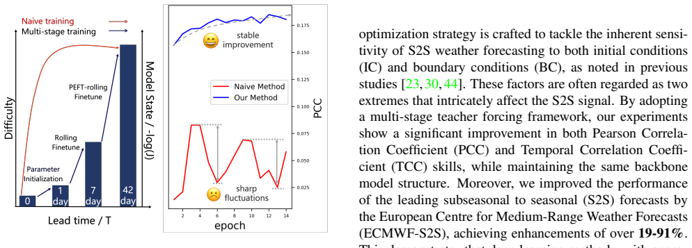
The load-bearing mechanism is the multi-stage teacher forcing training schedule, understood through error accumulation in rolling prediction. When a model rolls forward, the parameter gradient contains products of Jacobians, $\prod_{k=j+1}^{T} J_k$, so any local parameter update is amplified or damped by the spectral growth of these products along the orbit, quantified by the maximum Lyapunov exponent $\lambda_{\max}$; in chaotic systems a positive $\lambda_{\max}$ produces diverging loss gradients. The recipe attacks this in three moves: it grows the rolling horizon in stages, $T = 1$, then $T = 7$, then $T = 42$, so each stage starts from a state with smaller Jacobians; it substitutes observed values for model predictions at controlled frequencies so the multiplicative path of the Jacobians is interrupted; and it freezes most parameters in the final stage, keeping only six adapter modules, one per seven-day block, trainable. The loss functions are computed on anomalies relative to an 11-day centered rolling climatology and combine latitude-weighted MSE with latitude-weighted Pearson correlation.
What would settle it
Recompute both systems' skill on a single shared anomaly baseline by applying the same 11-day centered rolling climatology from the same reference period to the model's forecasts, ERA5, and the ECMWF-S2S reforecasts, and check whether the 19-91% advantage in PCC and TCC survives; also recompute the headline averages over all ten modeled variables, including total precipitation, rather than the six reported ones.
Extended reading notes
Core claim
The paper's central claim is that optimization, not network structure, is the deciding factor in whether deep learning succeeds at subseasonal-to-seasonal forecasting. Using a fixed backbone, a Siamese-MAE-pretrained vision transformer, the authors show that training a 42-day rolling predictor end to end is unstable because the backpropagation path contains products of Jacobian matrices along the forecast orbit, whose growth is controlled by the orbit's maximum Lyapunov exponent. Their remedy is a three-stage curriculum: fine-tune the model as a one-day forecaster, then as a seven-day roller, then as a 42-day roller with parameter-efficient adapters, while teacher forcing substitutes observed values for predictions at intermediate steps to break the multiplicative path of the Jacobians. On latitude-weighted anomaly correlations for six variables, t2m, z500, t850, olr, u200, and u850, the resulting model outperforms the ECMWF-S2S system by 19-91% over the 2-to-6-week window and extends skillful MJO prediction from 23 to 30 days. The paper further claims that rolling forecasting trained this way beats direct forecasting by over 30%, directly contesting the ChaosBench finding that direct forecasting is superior for S2S.
Load-bearing premise
The headline claim that the model beats ECMWF-S2S by 19-91% assumes the two systems are scored on comparable anomaly baselines: the paper's own forecasts use an 11-day centered rolling climatology while ECMWF's published skill uses ECMWF's own climatology, and the paper itself warns that a different or longer climatology window can make apparent skill look inflated.
Editorial extensions
If this is right
- Existing deep learning weather models that score at climatology level for 2-6 week leads could be upgraded to subseasonal skill by retraining with the multi-stage teacher forcing schedule, with no change to their architecture.
- The benchmark conclusion that direct forecasting beats rolling forecasting for S2S would need revision, since rolling predictors trained this way win by over 30% on correlation skills and the comparison in that benchmark is confounded by how the rolling models were optimized.
- Operational S2S forecasting could shift from running costly physics-based ensemble systems to much cheaper learned models, at least for the six large-scale variables studied.
- The curriculum idea of gradually lengthening the prediction horizon while injecting ground truth transfers to any iterative spatiotemporal predictor, including other weather backbones and climate emulators.
Reading between the lines
- The reported 19-91% margin may owe part of its size to a scoring asymmetry: the paper's own anomaly skill is computed against a sharp 11-day rolling climatology while ECMWF's skill figures use a fixed climatology, and the paper's own evaluation section warns that fixed or longer climatologies weaken the anomaly signal and can inflate apparent gains; a fair head-to-head needs a shared anomaly basel
- The headline averages exclude four of the ten modeled variables, including total precipitation, which is typically among the hardest subseasonal targets, so the claim that deep learning surpasses ECMWF-S2S should be read as applying to the six selected variables.
- The Jacobian-product analysis justifies the training schedule through a linearized model, but the paper does not directly measure the spectral norm of the actual network Jacobians; a natural test is to record $\| \prod J_k \|_2$ at each training stage and check that it decreases as the schedule progresses.
- If the optimization-centered explanation is right, the current S2S skill ceiling is set by training difficulty rather than by expressivity or data, which predicts that applying this recipe to stronger backbones listed in the paper, such as GraphCast or Pangu-Weather, would yield further gains, a direct extension the paper leaves to future work.
Editorial analysis
A structured set of objections, weighed in public.
Referee Report
Summary. The paper argues that the poor performance of deep learning models at subseasonal-to-seasonal (S2S) forecasting is caused by the optimization procedure rather than by the model architecture. The authors propose a multi-stage teacher-forcing training scheme that first fine-tunes a pretrained 'Baguan' backbone to a 1-day forecast, then to a 7-day rolling horizon, and finally to a 42-day rolling horizon with adapter-based PEFT, using anomaly-based losses. They report that this scheme, with the same backbone, surpasses ECMWF-S2S by 19-91% in PCC and TCC, extends the skillful MJO forecast lead time from 23 to 30 days, and reverses the ChaosBench conclusion that direct forecasting outperforms rolling forecasting. A theoretical analysis based on deep linear models and Jacobian accumulation is included to explain why the curriculum-style training helps.
Significance. If the claims are substantiated, the paper would make an important contribution: it would show that a training recipe alone can push existing deep-learning architectures to S2S skill beyond a leading NWP system, and it would challenge a recent benchmark finding. The manuscript has concrete strengths: it ships an implementation, provides ablations over two backbones and two resolutions, and formulates a falsifiable claim about rolling versus direct forecasting. However, the headline results currently rest on a non-apples-to-apples evaluation (different climatology conventions), a selected variable subset, and unquantified run-to-run variability, so the significance cannot be fully assessed at this stage.
major comments (5)
- [§4.1.2 and §4.2] The headline comparison with ECMWF-S2S is computed under two different anomaly baselines: the model and ERA5 use an 11-day centered rolling climatology, while ECMWF uses its own climatology, and the paper itself warns that 'using a longer average or fixed time period can weaken the climatology signal, making the results appear inflated.' Because PCC and TCC are correlations of anomalies, this difference directly changes the scores; without a sensitivity experiment in which ECMWF skill is recomputed with the same ERA5 climatology (or the model with ECMWF's), the reported 19–91% improvement cannot be attributed to forecast quality rather than scoring convention. This is load-bearing because the abstract, introduction, and conclusion all present the ECMWF comparison as the primary evidence for the 'optimization, not architecture' thesis.
- [§4.1.2 and §4.2] The stated 'over 19–91%' improvement is averaged over only 6 of the 10 modeled variables: t2m, z500, t850, olr, u200, and u850. The paper says these are 'primarily reported' because of 'importance of the signals,' but total precipitation (tp) and the other humidity and wind variables are excluded from the headline skill numbers; this is a selection on the outcome and can inflate the perceived improvement. The authors should report skill for all variables they claim to forecast or provide a principled reason for the subset and show that the conclusion is not sensitive to the choice.
- [§3 (Figure 3) and §5] The claim that the multi-stage rolling method outperforms direct forecasting by 'over 30%' is stated in the abstract and introduction, but the experimental section does not quantify this comparison: Figure 3 is illustrative, and the ablations in §5 compare only rolling variants (our method versus the naive method), not against direct forecasting models. Without a table or figure showing actual PCC and TCC values for direct forecasting under the same conditions, the challenge to the ChaosBench conclusion is not supported by the presented evidence.
- [Appendix B, Eqs. (8)–(14)] The theoretical explanation rests on inequality (8), |∇ℓ(Θ)|² ≥ 4L² ℓ(Θ)(1 − σ_min(Θ)), which is asserted as 'easy to verify' with no proof and no explicit statement of which lemma from the original paper is being modified. This inequality drives the convergence bound (14); if it is not established, the theoretical rationale for why curriculum-style training reduces optimization difficulty is unsupported. The authors need to provide a complete proof or a precise citation that contains this exact inequality.
- [§4.2 and §5] The paper reports no error bars, confidence intervals, or significance tests for any of the skill metrics, and the claims of 'significantly improves' and 'surpassing' are based on single training runs for each configuration. The differences in Table 1 (e.g., ViT 0.1168 versus 0.0807) are small in absolute PCC units, so a statement of run-to-run variability is necessary to judge whether the reported gains are reproducible and not due to training noise.
minor comments (6)
- [§3.2 and Reference [1]] The 'Baguan' backbone is described only through a non-archival blog link; the paper should include a full architectural description or cite a peer-reviewed/preprint source so that the base model is reproducible.
- [§4.1.1] For stage 1, the peak and minimum learning rates are both given as 1e−4, so the schedule is constant; please state this explicitly to avoid confusion.
- [Table 1] The 'Depth' column (51*42 and 15*42) is undefined; clarify how depth is computed and why it is reported as the product of network depth and rollout length.
- [§4.3] The MJO evaluation uses only the year 2015; state whether this is the standard verification period and whether the result is stable across other years.
- [Figures 5 and 6] The captions contain a spelling error ('comparsion'); also, the figures would benefit from axis labels defining the lead time range and the metric unit.
- [§3.2] The text in the loss-function paragraph says 'we use use A to denote anomaly values' — the duplicated 'use' should be removed.
Circularity Check
No circular derivation: the multi-stage optimization claim is tested against external baselines and controlled ablations; the only same-group citation (Baguan backbone) is not load-bearing.
full rationale
I walked the claimed derivation chain. The central empirical claim is not circular: the multi-stage teacher-forcing schedule (T = 1, 7, 42, Sec. 3.2) is a training strategy, and its gains are measured against the naive 42-day fine-tune (Sec. 5.1, Table 1), direct forecasting (Fig. 3), and external ECMWF-S2S (Sec. 4.2). No fitted parameter is renamed as a prediction; the ablations hold the backbone fixed and vary only the optimization, so 'optimization, not architecture' is a controlled comparison. The theoretical motivation (Sec. 3.1) is the exact BPTT chain-rule identity containing products of Jacobians, which is standard calculus; the instability statement is explicitly supported by external reference [24], and Appendix B says 'Our analysis follows closely the work' of Bartlett et al. [2], adding 'we can follow the identical analysis from the original work.' That is a derivative analogy, not a self-referential proof. The one same-group citation is the Baguan pretrained backbone [1], a non-archival DAMO Academy blog; it supplies model weights rather than an argument, and the controlled experiments use identical weights for the compared training methods, so no result reduces to the citation. Two non-circular weaknesses deserve explicit flagging: (i) Sec. 4.1.2 scores model anomalies with an 11-day centered ERA5 climatology while 'ECMWF employs its own climatology,' and then warns that 'using a longer average or fixed time period can weaken the climatology signal, making the results appear inflated'; the headline 19-91% margin is therefore a benchmark-comparability risk, not a circularity; (ii) the same section defines climatology as 'the average values for each day of the year across all years,' potentially including test years, which is a leakage risk. Both are correctness concerns, not cases where the prediction equals its input by construction. Score 2 reflects the minor non-load-bearing self-citation only.
Assumptions & free parameters
free parameters (4)
- Stage-wise peak and minimum learning rates =
1e-4/1e-4, 2e-6/1e-6, 2e-6/1e-6
- Rolling horizon schedule (T = 1, 7, 42) =
1 day, 7 days, 42 days
- Number of adapter sets and adapter size =
6 sets, each 4% of parameters, hidden dim 1024
- Climatology averaging window =
11-day centered rolling mean
assumptions (5)
- standard math BPTT gradient formula for the rolling RNN (page 3): gradient is a sum of products of Jacobians J_k along the trajectory.
- domain assumption Positive maximum Lyapunov exponent lambda_max > 0 leads to diverging loss gradients when training RNNs on chaotic series with gradient descent.
- ad hoc to paper Deep-linear-model analysis in Appendix B: inequality (8), |grad ell|^2 >= 4 L^2 ell(Theta) (1 - sigma_min(Theta)), is asserted as 'easy to verify' and then drives the convergence bound (14).
- domain assumption ERA5 reanalysis is treated as ground truth for training and verification.
- domain assumption ECMWF-S2S reforecasts (C47r3) are a fair operational baseline, and computing ECMWF's climatology over 2002-2021 while testing on 2015-2018 is acceptable.
Cite this review
Pith. "Pith review of Maximizing the Impact of Deep Learning on Subseasonal-to-Seasonal Climate Forecasting: The Essential Role of Optimization." pith.science (2026). https://pith.science/paper/L4IIFK3K
@misc{pith2026241116728,
  author       = {Pith},
  title        = {Pith review of: Maximizing the Impact of Deep Learning on Subseasonal-to-Seasonal Climate Forecasting: The Essential Role of Optimization},
  year         = {2026},
  howpublished = {\url{https://pith.science/paper/L4IIFK3K}},
  note         = {Machine review of arXiv:2411.16728}
}
read the original abstract
Weather and climate forecasting is vital for sectors such as agriculture and disaster management. Although numerical weather prediction (NWP) systems have advanced, forecasting at the subseasonal-to-seasonal (S2S) scale, spanning 2 to 6 weeks, remains challenging due to the chaotic and sparse atmospheric signals at this interval. Even state-of-the-art deep learning models struggle to outperform simple climatology models in this domain. This paper identifies that optimization, instead of network structure, could be the root cause of this performance gap, and then we develop a novel multi-stage optimization strategy to close the gap. Extensive empirical studies demonstrate that our multi-stage optimization approach significantly improves key skill metrics, PCC and TCC, while utilizing the same backbone structure, surpassing the state-of-the-art NWP systems (ECMWF-S2S) by over \textbf{19-91\%}. Our research contests the recent study that direct forecasting outperforms rolling forecasting for S2S tasks. Through theoretical analysis, we propose that the underperformance of rolling forecasting may arise from the accumulation of Jacobian matrix products during training. Our multi-stage framework can be viewed as a form of teacher forcing to address this issue. Code is available at \url{https://anonymous.4open.science/r/Baguan-S2S-23E7/}
Figures


Figures from the paper (16 more)


Reference graph
Works this paper leans on
-
[1]
Alibaba damo academy unveils advanced weather fore- casting model “baguan”. https://damo.alibaba. com / events / 32024110717309481802521085 ? language=en, 2024. Accessed: 2024-11-06. 4, 5
work page 2024
-
[2]
Peter Bartlett, Dave Helmbold, and Philip Long. Gradient descent with identity initialization efficiently learns positive definite linear transformations by deep residual networks. In International conference on machine learning , pages 521–
-
[3]
The quiet revolution of numerical weather prediction
Peter Bauer, Alan Thorpe, and Gilbert Brunet. The quiet revolution of numerical weather prediction. Nature, 525(7567):47–55, 2015. 1
work page 2015
-
[4]
Yoshua Bengio, J ´erˆome Louradour, Ronan Collobert, and Ja- son Weston. Curriculum learning. InProceedings of the 26th annual international conference on machine learning, pages 41–48, 2009. 4
work page 2009
-
[5]
Pangu-weather: A 3d high-resolution model for fast and accurate global weather forecast
Kaifeng Bi, Lingxi Xie, Hengheng Zhang, Xin Chen, Xiao- tao Gu, and Qi Tian. Pangu-weather: A 3d high-resolution model for fast and accurate global weather forecast. arXiv preprint arXiv:2211.02556, 2022. 2, 3
arXiv 2022
-
[6]
Bruinsma, Ana Lucic, Megan Stanley, Johannes Brandstetter, Patrick Garvan, Maik Riechert, Jonathan A
Cristian Bodnar, Wessel P. Bruinsma, Ana Lucic, Megan Stanley, Johannes Brandstetter, Patrick Garvan, Maik Riechert, Jonathan A. Weyn, Haiyu Dong, Anna Vaughan, Jayesh K. Gupta, Kit Thambiratnam, Alex Archibald, Eliz- abeth Heider, Max Welling, Richard E. Turner, and Paris Perdikaris. Aurora: A foundation model of the atmosphere. ArXiv, abs/2405.13063, 2024. 2
arXiv 2024
-
[7]
Spherical fourier neural operators: Learning stable dynamics on the sphere
Boris Bonev, Thorsten Kurth, Christian Hundt, Jaideep Pathak, Maximilian Baust, Karthik Kashinath, and Anima Anandkumar. Spherical fourier neural operators: Learning stable dynamics on the sphere. In International Conference on Machine Learning, 2023. 2, 3
work page 2023
-
[8]
J. Buch, A. P. Williams, C. S. Juang, W. D. Hansen, and P. Gentine. Smlfire1.0: a stochastic machine learning (sml) model for wildfire activity in the western united states. Geo- scientific Model Development, 16(12):3407–3433, 2023. 1
work page 2023
Show all 46 references
-
[9]
Fengwu: Pushing the skillful global medium-range weather forecast beyond 10 days lead
Kan Chen, Tao Han, Junchao Gong, Lei Bai, Fenghua Ling, Jingyao Luo, Xi Chen, Lei Ma, Tianning Zhang, Rui Su, Yuanzheng Ci, Bin Li, Xiaokang Yang, and Wanli Ouyang. Fengwu: Pushing the skillful global medium-range weather forecast beyond 10 days lead. ArXiv, abs/2304.02948, 2023. 2
2023
-
[10]
Fuxi: a cascade machine learning forecasting system for 15-day global weather fore- cast
Lei Chen, Xiaohui Zhong, Feng jun Zhang, Yuan Cheng, Yinghui Xu, Yuan Qi, and Hao Li. Fuxi: a cascade machine learning forecasting system for 15-day global weather fore- cast. npj Climate and Atmospheric Science, 6:1–11, 2023. 2, 3
2023
-
[11]
Fuxi-s2s: An accurate machine learn- ing model for global subseasonal forecasts
Lei Chen, Xiaohui Zhong, Jie Wu, Deliang Chen, Shang- ping Xie, Qingchen Chao, Chensen Lin, Zixin Hu, Bo Lu, Hao Li, et al. Fuxi-s2s: An accurate machine learn- ing model for global subseasonal forecasts. arXiv preprint arXiv:2312.09926, 2023. 2, 3
2023 arXiv
-
[12]
Fundamentals of numerical weather predic- tion
Jean Coiffier. Fundamentals of numerical weather predic- tion. Cambridge University Press, 2011. 1
2011
-
[13]
An image is worth 16x16 words: Transformers for image recognition at scale
Alexey Dosovitskiy. An image is worth 16x16 words: Transformers for image recognition at scale. arXiv preprint arXiv:2010.11929, 2020. 7
2010 arXiv
-
[14]
Siamese masked autoencoders
Agrim Gupta, Jiajun Wu, Jia Deng, and Fei-Fei Li. Siamese masked autoencoders. Advances in Neural Information Pro- cessing Systems, 36:40676–40693, 2023. 4, 5
2023
-
[15]
The era5 global reanalysis
Hans Hersbach, Bill Bell, Paul Berrisford, Shoji Hirahara, Andr´as Hor ´anyi, Joaqu ´ın Mu ˜noz-Sabater, Julien Nicolas, Carole Peubey, Raluca Radu, Dinand Schepers, et al. The era5 global reanalysis. Quarterly Journal of the Royal Mete- orological Society, 146(730):1999–2049, 2020. 5
1999
-
[16]
Generalized teacher forcing for learning chaotic dynamics
Florian Hess, Zahra Monfared, Manuel Brenner, and Daniel Durstewitz. Generalized teacher forcing for learning chaotic dynamics. arXiv preprint arXiv:2306.04406, 2023. 3, 4
2023 arXiv
-
[17]
Parameter-efficient transfer learning for nlp
Neil Houlsby, Andrei Giurgiu, Stanislaw Jastrzebski, Bruna Morrone, Quentin De Laroussilhe, Andrea Gesmundo, Mona Attariyan, and Sylvain Gelly. Parameter-efficient transfer learning for nlp. In International conference on machine learning, pages 2790–2799. PMLR, 2019. 5
2019
-
[18]
The platonic representation hypothesis
Minyoung Huh, Brian Cheung, Tongzhou Wang, and Phillip Isola. The platonic representation hypothesis. arXiv preprint arXiv:2405.07987, 2024. 5
2024 arXiv
-
[19]
Auto-encoding variational bayes
Diederik P Kingma. Auto-encoding variational bayes. arXiv preprint arXiv:1312.6114, 2013. 3
2013 arXiv
-
[20]
Similarity of neural network represen- tations revisited
Simon Kornblith, Mohammad Norouzi, Honglak Lee, and Geoffrey Hinton. Similarity of neural network represen- tations revisited. In International conference on machine learning, pages 3519–3529. PMLR, 2019. 5
2019
-
[21]
Learning skillful medium-range global weather forecasting
Remi Lam, Alvaro Sanchez-Gonzalez, Matthew Willson, Peter Wirnsberger, Meire Fortunato, Ferran Alet, Suman Ravuri, Timo Ewalds, Zach Eaton-Rosen, Weihua Hu, Alexander Merose, Stephan Hoyer, George Holland, Oriol Vinyals, Jacklynn Stott, Alexander Pritzel, Shakir Mohamed, and P...
2023
-
[22]
Analysis methods for numerical weather prediction
Andrew C Lorenc. Analysis methods for numerical weather prediction. Quarterly Journal of the Royal Meteorological Society, 112(474):1177–1194, 1986. 1
1986
-
[23]
Deterministic nonperiodic flow
Edward N Lorenz. Deterministic nonperiodic flow. Journal of atmospheric sciences, 20(2):130–141, 1963. 1, 2
1963
-
[24]
On the difficulty of learning chaotic dynamics with rnns
Jonas Mikhaeil, Zahra Monfared, and Daniel Durste- witz. On the difficulty of learning chaotic dynamics with rnns. Advances in Neural Information Processing Systems , 35:11297–11312, 2022. 4
2022
-
[25]
Adaptive bias correction for im- proved subseasonal forecasting
Soukayna Mouatadid, Paulo Orenstein, Genevieve Flaspohler, Judah Cohen, Miruna Oprescu, Ernest Fraenkel, and Lester Mackey. Adaptive bias correction for im- proved subseasonal forecasting. Nature Communications , 14(1):3482, 2023. 2
2023
-
[26]
Chaosbench: A multi-channel, physics-based benchmark for subseasonal-to-seasonal climate prediction
Juan Nathaniel, Yongquan Qu, Tung Nguyen, Sungduk Yu, Julius Busecke, Aditya Grover, and Pierre Gentine. Chaosbench: A multi-channel, physics-based benchmark for subseasonal-to-seasonal climate prediction. arXiv preprint arXiv:2402.00712, 2024. 2, 3, 8
2024 arXiv
-
[27]
Gupta, and Aditya Grover
Tung Nguyen, Johannes Brandstetter, Ashish Kapoor, Jayesh K. Gupta, and Aditya Grover. Climax: A foundation model for weather and climate. In International Conference on Machine Learning, 2023. 2, 3
2023
-
[28]
Fourcastnet: A global data-driven high- resolution weather model using adaptive fourier neural op- erators
Jaideep Pathak, Shashank Subramanian, Peter Harrington, Sanjeev Raja, Ashesh Chattopadhyay, Morteza Mardani, Thorsten Kurth, David Hall, Zongyi Li, Kamyar Azizzade- nesheli, et al. Fourcastnet: A global data-driven high- resolution weather model using adaptive fourier neural o...
2022 arXiv
-
[29]
Pendergrass, Gerald A
Angeline G. Pendergrass, Gerald A. Meehl, Roger Pul- warty, Mike Hobbins, Andrew Hoell, Amir AghaKouchak, C´eline J. W. Bonfils, Ailie J. E. Gallant, Martin Hoer- ling, David Hoffmann, Laurna Kaatz, Flavio Lehner, Dag- mar Llewellyn, Philip Mote, Richard B. Neale, Jonathan T. ...
2020
-
[30]
The role of model and initial condition error in numerical weather forecasting in- vestigated with an observing system simulation experiment
Nikki Priv ´e and RONALD Errico. The role of model and initial condition error in numerical weather forecasting in- vestigated with an observing system simulation experiment. Tellus, 65, 11 2013. 1, 2
2013
-
[31]
U- net: Convolutional networks for biomedical image segmen- tation
Olaf Ronneberger, Philipp Fischer, and Thomas Brox. U- net: Convolutional networks for biomedical image segmen- tation. In Medical image computing and computer-assisted intervention–MICCAI 2015: 18th international conference, Munich, Germany, October 5-9, 2015, proceedings, pa...
2015
-
[32]
Learning representations by back-propagating er- rors
David E Rumelhart, Geoffrey E Hinton, and Ronald J Williams. Learning representations by back-propagating er- rors. nature, 323(6088):533–536, 1986. 3
1986
-
[33]
The ncep climate forecast system version 2
Suranjana Saha, Shrinivas Moorthi, Xingren Wu, Jiande Wang, Sudhir Nadiga, Patrick Tripp, David Behringer, Yu- Tai Hou, Hui-ya Chuang, Mark Iredell, et al. The ncep climate forecast system version 2. Journal of climate , 27(6):2185–2208, 2014. 3
2014
-
[34]
Lamb, Yu Huang, and Pierre Gen- tine
Sara Shamekh, Kara D. Lamb, Yu Huang, and Pierre Gen- tine. Implicit learning of convective organization explains precipitation stochasticity. Proceedings of the National Academy of Sciences, 120(20):e2216158120, 2023. 1
2023
-
[35]
Climode: Climate and weather forecasting with physics-informed neu- ral odes
Yogesh Verma, Markus Heinonen, and Vikas Garg. Climode: Climate and weather forecasting with physics-informed neu- ral odes. arXiv preprint arXiv:2404.10024, 2024. 3
2024 arXiv
-
[36]
Evolution of ecmwf sub-seasonal forecast skill scores
Fr ´ed´eric Vitart. Evolution of ecmwf sub-seasonal forecast skill scores. Quarterly Journal of the Royal Meteorological Society, 140(683):1889–1899, 2014. 3
2014
-
[37]
The sub-seasonal to seasonal prediction project (s2s) and the prediction of ex- treme events
Frederic Vitart and Andrew Robertson. The sub-seasonal to seasonal prediction project (s2s) and the prediction of ex- treme events. npj Climate and Atmospheric Science , 1, 03
-
[38]
Subseasonal to seasonal prediction project: Bridging the gap between weather and climate
Fr ´ed´eric Vitart, Andrew W Robertson, and David LT Ander- son. Subseasonal to seasonal prediction project: Bridging the gap between weather and climate. Bulletin of the World Meteorological Organization, 61(2):23, 2012. 1
2012
-
[39]
Backpropagation through time: what it does and how to do it
Paul J Werbos. Backpropagation through time: what it does and how to do it. Proceedings of the IEEE , 78(10):1550– 1560, 1990. 3
1990
-
[40]
An all-season real-time multivariate mjo index: Development of an in- dex for monitoring and prediction
Matthew C Wheeler and Harry H Hendon. An all-season real-time multivariate mjo index: Development of an in- dex for monitoring and prediction. Monthly weather review, 132(8):1917–1932, 2004. 7
1917
-
[41]
Potential applications of subseasonal-to-seasonal (s2s) predictions
Christopher J White, Henrik Carlsen, Andrew W Robertson, Richard JT Klein, Jeffrey K Lazo, Arun Kumar, Frederic Vi- tart, Erin Coughlan de Perez, Andrea J Ray, Virginia Mur- ray, et al. Potential applications of subseasonal-to-seasonal (s2s) predictions. Meteorological applica...
2017
-
[42]
The met office global coupled model 2.0 (gc2) con- figuration
KD Williams, CM Harris, A Bodas-Salcedo, J Camp, RE Comer, D Copsey, D Fereday, T Graham, R Hill, T Hinton, et al. The met office global coupled model 2.0 (gc2) con- figuration. Geoscientific Model Development, 88(55):1509– 1524, 2015. 3
2015
-
[43]
The beijing climate center climate system model (bcc-csm): The main progress from cmip5 to cmip6
Tongwen Wu, Yixiong Lu, Yongjie Fang, Xiaoge Xin, Lau- rent Li, Weiping Li, Weihua Jie, Jie Zhang, Yiming Liu, Li Zhang, et al. The beijing climate center climate system model (bcc-csm): The main progress from cmip5 to cmip6. Geoscientific Model Development , 12(4):1573–1600, 2019. 3
2019
-
[44]
Estimating the uncertainty in a regional climate model related to initial and lateral boundary conditions
Wanli Wu and Aaron Rivers. Estimating the uncertainty in a regional climate model related to initial and lateral boundary conditions. Journal of Climate - J CLIMATE , 18:917–933, 04 2005. 1, 2
2005
-
[45]
Vargas Zeppetello, David S
Lucas R. Vargas Zeppetello, David S. Battisti, and Mar- cia B. Baker. The physics of heat waves: What causes ex- tremely high summertime temperatures? Journal of Climate, 35(7):2231 – 2251, 2022. 1 10 Appendix A. Resource Open Sourcing Our method and codes are open-sourced at ...
2022
-
[46]
Gradient descent with identity initialization efficiently learns positive definite linear trans- formations by deep residual networks
In this note, we consider a spe- cial case of deep linear model that has Θi = Θ, i∈ [L]. It fits in better with the rolling out method in our study where the same model is used at every step of rolling out. We will show that in order to achieve a fast convergence of deep linea...
Reviewed August 12, 2026 · model on record in the stance chip above.
Discussion (0). Continue with ORCID to comment.