REVIEW 3 major objections 6 minor 41 references
MiceBoneChallenge: Micro-CT public dataset and six solutions for automatic growth plate detection in micro-CT mice bone scans
T0 review · 3 major / 6 minor · reviewed 2026-08-12 · deepseek-v4-flash
Pith's one-line read This paper claims that mouse bone growth plates can be located automatically in 3D micro-CT scans with a mean error of about two image planes, and it releases the first public annotated dataset and six deep-learning solutions to make this…
desk verdict Useful dataset-and-benchmark paper for mouse micro-CT growth plate detection; the headline MAE is internally consistent, but the single-expert ground truth and the missing absolute value in Eq. 1 weaken the 'radiologist-acceptable' claim. read the letter →
The pith
A machine-rendered reading of the paper's core claim, the machinery that carries it, and where it could break.
The reading
What carries the argument
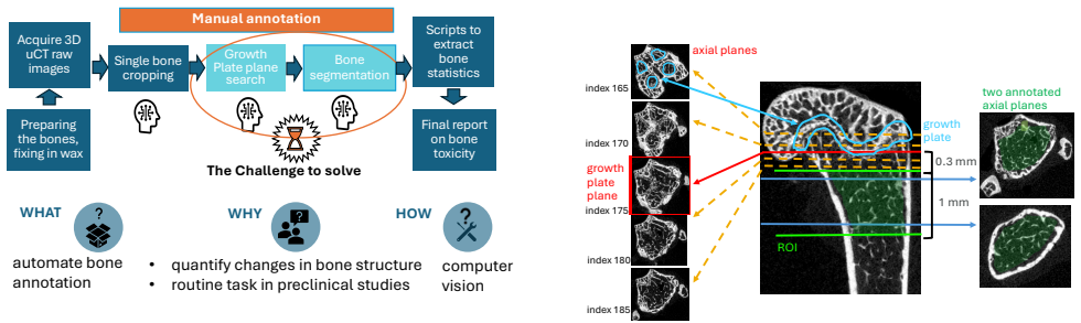
The central object is the growth plate plane index (GPPI), defined as the lowest axial plane of the femoral growth plate where the four protrusions of the bone head merge; it anchors the volume of interest for trabecular bone measurement, a 1-mm cylinder starting 0.3 mm distal to the plane. The carried argument is a challenge comparison: six teams solve GPPI prediction using three architectural families: a 3D sliding-window ResNet34 with a decoupled classification and regression head, 2.5D EfficientNet regressions over stacked sagittal and coronal slices, and 2D axial-plane binary classifiers with morphological post-processing to clean the before/after decision boundary. Performance is scored with a scaled survival function, $\mathrm{Score} = 2\bar{\Phi}((p-t)/3)$, which maps a zero-plane error to score 1 and decays smoothly toward 0 as the prediction-to-truth distance grows.
What would settle it
Re-annotate the 13 test scans, or a random subset of the 83, with a second independent expert and compute inter-observer plane-index disagreement. If expert-against-expert differences have a mean absolute value near 2 planes, comparable to the best models' MAE, then the reported accuracy cannot be separated from annotation noise, and the ranking among teams would be reshuffled by which expert's labels define ground truth.
Extended reading notes
Core claim
The central claim is that bone-growth-plate identification in rodent micro-CT, a prerequisite for automated trabecular bone quantification, can be automated to an accuracy acceptable for practical use by a radiologist. The authors organize the claim around a new resource: 83 annotated 3D $\mu$CT femur scans, with growth plate plane indices (GPPI) labeled by an expert with 20 years of experience and quality-checked by a second expert, plus the code, models, and pixel-wise bone segmentations. Six independent challenge solutions, spanning 3D sliding-window CNN regression, 2.5D long-axis regression, and 2D axial-plane classification, achieve per-team mean absolute errors from 1.23 to 3.62 planes on the test set, with a pooled mean of $1.91 \pm 0.87$ planes. Notably, full-3D convolution did not outperform simpler 2.5D stacking approaches. The authors' intended contribution is therefore both a benchmark dataset and a demonstration that this previously manual landmark-detection task can be solved with accessible deep-learning pipelines.
Load-bearing premise
The load-bearing premise is that the single expert's manual growth-plate labels are correct and reproducible enough to serve as ground truth; the paper reports no inter- or intra-observer variability, so every error and ranking is measured against an unexamined target.
Editorial extensions
If this is right
- A public benchmark for growth-plate detection in mouse femurs now exists, with 83 annotated volumes, code, and trained models released for direct comparison.
- With planes 10 $\mu$m apart, a mean absolute error of 1.91 planes moves the volume-of-interest start by roughly 19 $\mu$m, which is small compared to the 1-mm analysis volume and supports the authors' practical-usability claim.
- The observation that 2.5D and 2D approaches match full-3D accuracy means preclinical labs without large GPU budgets can adopt the cheaper pipelines.
- Because pixel-wise bone segmentations are included, the dataset also supports the downstream segmentation task, enabling end-to-end automated bone quantification.
- Six of the 23 challenge teams delivered final solutions, and their methods span three distinct modeling families, giving future participants a documented starting point.
Reading between the lines
- Editorial inference: because annotation noise is unmeasured, the best models' MAE of 1.23 to 1.91 planes may already be at the noise floor of the ground truth; a direct test is to compare model predictions against a second expert's re-annotation of the same scans.
- Editorial inference: the two-stage design in the better 2.5D solutions (coarse long-axis localization followed by fine cropped regression) suggests that a hybrid coarse-to-fine pipeline could push error below one plane, a possibility the paper notes but does not test.
- Editorial inference: the claimed clinical acceptability could be verified end-to-end by computing trabecular bone volume fraction from manual versus predicted GPPI on the same scans and checking whether the derived endpoints differ by less than the $\pm 10\%$ drug-effect threshold the paper cites as decision-relevant.
- Editorial inference: the released dataset comes from three preclinical studies on one scanner, so cross-scanner and cross-strain generalization remains open; a natural extension is fine-tuning on tibia or vertebra scans or on images from a different $\mu$CT system.
Editorial analysis
A structured set of objections, weighed in public.
Referee Report
Summary. The paper describes MiceBoneChallenge, an internal challenge organized at a pharmaceutical company to automate growth plate plane detection in micro-CT scans of mouse femurs. The authors release a dataset of 83 annotated 3D scans, present six deep learning solutions spanning 3D regression, 2.5D long-axis regression, and 2D axial classification, and report a collective mean absolute error of 1.91 ± 0.87 planes on a 13-scan test set, which they state is acceptable for practical use by a radiologist. The data, code, and trained models are promised to be made public.
Significance. If the dataset and annotations are released as promised, this is a useful contribution: it addresses a real gap in public preclinical micro-CT datasets for rodent bone growth plate detection and provides six independently implemented baselines with shared code. The reported performance numbers are internally consistent: the score sums in Table 6 match absolute-error scoring with a survival function, and the per-team MAEs in Table 5 are plausible. The main limitations are the absence of ground-truth label variability quantification and the small test set, both of which currently temper the strength of the accuracy and ranking claims.
major comments (3)
- [§3.3.1, Eq. (1)] The evaluation score is defined as 2Φ̄((p − t)/3) without an absolute value. As written, a prediction below the true plane (p < t) produces a negative argument to the CCDF and hence a score greater than 1; for example, an error of −3 planes gives a score of about 1.68, contradicting Table 1 and the stated [0, 1] range. The numerical results in Table 6 are consistent with 2Φ̄(|p − t|/3), so the intended metric is recoverable, but the equation and surrounding text should be corrected to avoid ambiguity in the central evaluation metric.
- [§3.2 and §6] The ground-truth GPPI was annotated by a single domain expert with quality control by another expert, but no inter- or intra-observer variability is reported. The GPP definition is subtle (Section 3.1, where adjacent planes are described as distinguishable only by experienced radiologists), and the paper's own motivation emphasizes eliminating observer variability. Without a repeatability study or a human-reader baseline, the reported MAE values and team rankings are measured against an uncharacterized target, and the abstract's claim that 1.91 ± 0.87 planes is 'acceptable for practical use by a radiologist' is not anchored. The Discussion already concedes that precise acceptable error rates still need to be established; please either provide label-variability data or temper the acceptability claim in the abstract and conclusions.
- [§5.1, Tables 5–6] The test set contains only 13 scans, and the differences among the top-ranked teams are small relative to the per-bone score variability. For instance, SN and BM have sum scores of 9.068 and 9.059, while the per-bone standard deviations are around 0.3, implying a standard error of roughly 0.08 on the sum; the observed difference is within noise. The paper should provide confidence intervals, bootstrap estimates, or a significance test for the team ranking, or explicitly state that the ranking is not statistically meaningful.
minor comments (6)
- [Abstract and §7] The abstract and conclusions state that the accuracy is 'acceptable for practical use by a radiologist,' while Section 6 refers to 'Anonymous Company's internal domain experts'; please align the terminology and avoid overclaiming.
- [Throughout] There are several typographical errors: 'utilzed' in Section 4.2.2, 'utlizing' in Section 4.2, 'ensambles' in Section 4.4, 'trainiable' in Supplementary Section 10.6.2, and 'the the GPP region' in Section 6.
- [Supplementary §10.2] Reference [12] (Lauterbur) is cited for µCT imaging; the appropriate citation for CT is Hounsfield [9], and the reference list should be checked for other citation mismatches.
- [Table 2 and Table 4] The resize dimension for Team SN is given as 321×244×244 in Table 2, while Table 4 lists the input size as 244×244×32; the relationship between these dimensions (downsampling followed by cropping) should be clarified.
- [§3.2] The text states that DICOM images use an 8-bit pixel format; micro-CT data are typically 16-bit, and if the data were converted to 8-bit, the paper should note whether and how this affects Hounsfield-unit precision for downstream bone quantification.
- [§4.5 and Supplementary §9] The abstract says the data 'will be shared' and the supplementary material provides an anonymized review link; for a dataset paper, a persistent DOI or a clear release license should be provided.
Circularity Check
No circularity: the reported accuracy is an empirical evaluation against a held-out test set, not a quantity derived from the models' own definitions.
full rationale
The paper reports a machine-learning challenge in which six teams trained models on a 70-scan training set and were evaluated on a 13-scan test set. The primary reported quantity, a mean absolute error of 1.91 ± 0.87 planes, is computed as the difference between model predictions and a manually annotated growth-plate-plane index (GPPI). The GPPI labels are independent of the models: they were produced by a domain expert before the challenge and served as the reference for both training and evaluation. There is no equation in the paper that defines the error metric in terms of the fitted parameters, and no fitted parameter is renamed as a prediction. The six solutions are genuinely empirical submissions; the paper does not claim to derive the GPPI from first principles. The statement that the accuracy is acceptable for practical use by a radiologist is an expert judgment, not a logical consequence of the models' construction, so it cannot be circular in the sense used here. The paper contains no load-bearing self-citation chain or imported uniqueness theorem; citations are to standard external methods (ResNet, EfficientNet, ImageNet, Albumentations, etc.). The main weakness, noted by the reader, is that the single-expert GPP annotation has no reported inter- or intra-observer variability, so the stability of the reference target is unquantified. That is a validity and reproducibility concern, not a circularity concern: the measurement pipeline is still external to the models and the test set is held out. Therefore no circular step can be exhibited, and the appropriate finding is no significant circularity with score 0.
Assumptions & free parameters
free parameters (5)
- Evaluation score decay scale (denominator 3 in Eq. 1) =
3
- SN regression loss weight lambda =
6
- CW bone cutoff threshold =
0.03
- MH input channel count and internal slice fraction =
9 channels; internal fraction tuned but value not reported
- Trained model weights of all six teams =
SN 63M, MH 12.2M, EK 4.2M, CW 11M, SV about 0.08M, BM 1.4M parameters
assumptions (4)
- domain assumption The growth plate plane is correctly defined as the lowest plane where the four femoral protrusions merge, and this is the appropriate landmark for defining the trabecular volume of interest.
- domain assumption Annotations from one expert with 20 years of experience, quality-controlled by another expert, form a reliable ground truth without quantified inter-observer variability.
- domain assumption The 13-bone test set is sufficient to rank methods and to support the stated practical accuracy.
- domain assumption A mean absolute error near 1.9 planes is acceptable for radiologist practice.
Cite this review
Pith. "Pith review of MiceBoneChallenge: Micro-CT public dataset and six solutions for automatic growth plate detection in micro-CT mice bone scans." pith.science (2026). https://pith.science/paper/UDEYJTNK
@misc{pith2026241117260,
  author       = {Pith},
  title        = {Pith review of: MiceBoneChallenge: Micro-CT public dataset and six solutions for automatic growth plate detection in micro-CT mice bone scans},
  year         = {2026},
  howpublished = {\url{https://pith.science/paper/UDEYJTNK}},
  note         = {Machine review of arXiv:2411.17260}
}
abstract
Detecting and quantifying bone changes in micro-CT scans of rodents is a common task in preclinical drug development studies. However, this task is manual, time-consuming and subject to inter- and intra-observer variability. In 2024, Anonymous Company organized an internal challenge to develop models for automatic bone quantification. We prepared and annotated a high-quality dataset of 3D $\mu$CT bone scans from $83$ mice. The challenge attracted over $80$ AI scientists from around the globe who formed $23$ teams. The participants were tasked with developing a solution to identify the plane where the bone growth happens, which is essential for fully automatic segmentation of trabecular bone. As a result, six computer vision solutions were developed that can accurately identify the location of the growth plate plane. The solutions achieved the mean absolute error of $1.91\pm0.87$ planes from the ground truth on the test set, an accuracy level acceptable for practical use by a radiologist. The annotated 3D scans dataset along with the six solutions and source code, is being made public, providing researchers with opportunities to develop and benchmark their own approaches. The code, trained models, and the data will be shared.
Figures


Figures from the paper (8 more)


Reference graph
Works this paper leans on
-
[1]
ML Bouxsein, SK Boyd, BA Christiansen, RE Guldberg, KJ Jepsen, and R M¨uller. Guidelines for assessment of bone mi- crostructure in rodents using micro-computed tomography.J Bone Miner Res., pages 1468–86, 2010. 1, 2
work page 2010
-
[2]
Iglovikov, Eugene Khved- chenya, Alex Parinov, Mikhail Druzhinin, and Alexandr A
Alexander Buslaev, Vladimir I. Iglovikov, Eugene Khved- chenya, Alex Parinov, Mikhail Druzhinin, and Alexandr A. Kalinin. Albumentations: Fast and flexible image augmen- tations. Information, 11(2), 2020. 3
work page 2020
-
[3]
Med3d: Transfer learning for 3d medical image analysis
Sihong Chen, Kai Ma, and Yefeng Zheng. Med3d: Transfer learning for 3d medical image analysis. ArXiv, abs/1904.00625, 2019. 1
arXiv 1904
-
[4]
B. Clarke. Normal bone anatomy and physiology. Clin J Am Soc Nephrol., pages 131–9, 2008. 1
work page 2008
- [5]
-
[6]
Imagenet: A large-scale hierarchical image database
Jia Deng, Wei Dong, Richard Socher, Li-Jia Li, Kai Li, and Li Fei-Fei. Imagenet: A large-scale hierarchical image database. In 2009 IEEE conference on computer vision and pattern recognition, pages 248–255. Ieee, 2009. 3
2009
-
[7]
Yolox: Exceeding yolo series in 2021, 2021
Zheng Ge, Songtao Liu, Feng Wang, Zeming Li, and Jian Sun. Yolox: Exceeding yolo series in 2021, 2021. 5
work page 2021
-
[8]
Deep residual learning for image recognition
Kaiming He, Xiangyu Zhang, Shaoqing Ren, and Jian Sun. Deep residual learning for image recognition. In Proceed- ings of the IEEE conference on computer vision and pattern recognition, pages 770–778, 2016. 6, 3
work page 2016
Show all 41 references
-
[9]
Computerized transverse axial scan- ning (tomography): Part 1
Godfrey N Hounsfield. Computerized transverse axial scan- ning (tomography): Part 1. description of system.The British journal of radiology, 46(552):1016–1022, 1973. 2
1973
-
[10]
Differenti- ation of distal ureteral stones and pelvic phleboliths using a convolutional neural network
Johan Jendeberg, Per Thunberg, and Mats Lid ´en. Differenti- ation of distal ureteral stones and pelvic phleboliths using a convolutional neural network. Urolithiasis, 49, 2021. 2
2021
-
[11]
Adam: A method for stochastic gradient descent
Diederik P Kingma and Jimmy Lei Ba. Adam: A method for stochastic gradient descent. In ICLR: international con- ference on learning representations, pages 1–15. ICLR US.,
-
[12]
Image formation by induced local inter- actions: Examples employing nuclear magnetic resonance
Paul C Lauterbur. Image formation by induced local inter- actions: Examples employing nuclear magnetic resonance. Nature, 242:190–191, 1973. 1
1973
-
[13]
Gradient-based learning applied to document recog- nition
Yann LeCun, L ´eon Bottou, Yoshua Bengio, and Patrick Haffner. Gradient-based learning applied to document recog- nition. Proceedings of the IEEE , 86(11):2278–2324, 1998. 1
1998
-
[14]
A survey on deep learning in medical image analysis
Geert Litjens, Thijs Kooi, Babak Ehteshami Bejnordi, Ar- naud Arindra Adiyoso Setio, Francesco Ciompi, Mohsen Ghafoorian, Jeroen Awm Van Der Laak, Bram Van Gin- neken, and Clara I S ´anchez. A survey on deep learning in medical image analysis. Medical image analysis, 42:60–88,
-
[15]
Decoupled weight decay regularization
I Loshchilov. Decoupled weight decay regularization. arXiv preprint arXiv:1711.05101, 2017. 3
2017 arXiv
-
[16]
Open-source pipeline for automatic segmenta- tion and microstructural analysis of murine knee subchondral bone
H Mahdi, M Hardisty, K Fullerton, K Vachhani, D Nam, and C Whyne. Open-source pipeline for automatic segmenta- tion and microstructural analysis of murine knee subchondral bone. Bone, page 116616, 2023. 2
2023
-
[17]
Neonatal retroviral vector-mediated hepatic gene therapy reduces bone, joint, and cartilage disease in mu- copolysaccharidosis vii mice and dogs
Robert Mango, Lingfei Xu, Mark Sands, Carole V ogler, Gabriela Seiler, Tobias Schwarz, Mark Haskins, and Kather- ine Ponder. Neonatal retroviral vector-mediated hepatic gene therapy reduces bone, joint, and cartilage disease in mu- copolysaccharidosis vii mice and dogs. Molecu...
2004
-
[18]
Neeteson, B.A
N.J. Neeteson, B.A. Besler, and D.E Whittier. Automatic segmentation of trabecular and cortical compartments in hr- pqct images using an embedding-predicting u-net and mor- phological post-processing. Sci Rep, page 116616, 2023. 2
2023
-
[19]
Automated microct- based bone and articular cartilage analysis using iterative shape averaging and atlas-based registration
Maerz T Newton MD, Junginger L. Automated microct- based bone and articular cartilage analysis using iterative shape averaging and atlas-based registration. Bone, page 115417, 2020. 2
2020
-
[20]
and et al
Yushkevich P. and et al. User-guided 3d active contour seg- mentation of anatomical structures: significantly improved efficiency and reliability.NeuroImage, 31(3):1116–28, 2006. 2
2006
-
[21]
Torchio: A python library for efficient loading, preprocessing, augmentation and patch-based sampling of medical images in deep learning
Fernando P ´erez-Garc´ıa, Rachel Sparks, and S ´ebastien Ourselin. Torchio: A python library for efficient loading, preprocessing, augmentation and patch-based sampling of medical images in deep learning. Computer Methods and Programs in Biomedicine, 208:106236, 2021. 1
2021
-
[22]
Micro-computed tomography reconstructions of tibiae of stem cell transplanted osteogenesis imperfecta mice
Anna Ranzoni, Michelangelo Corcelli, Tim Arnett, and Pas- cale Guillot. Micro-computed tomography reconstructions of tibiae of stem cell transplanted osteogenesis imperfecta mice. Scientific Data, 5:180100, 2018. 2
2018
-
[23]
S Rosenhain, ZA Magnuska, GG Yamoah, W A Rawashdeh, F Kiessling, and F. Gremse. A preclinical micro-computed tomography database including 3d whole body organ seg- mentations. Scientifc data, pages 1–9, 2018. 2
2018
-
[24]
J. Shim, C. Iwaya, C.G. Ambrose, and et al. Micro-computed tomography assessment of bone structure in aging mice.Sci- entific Reports, 12(1):1–12, 2022. 1
2022
-
[25]
Micro-computed tomography assessment of bone structure in aging mice
J Shim, C Iwaya, CG Ambrose, A Suzuki, and J Iwata. Micro-computed tomography assessment of bone structure in aging mice. Sci Rep, page 8117, 2022. 1
2022
-
[26]
Deep learning for automated skeletal bone age assessment in x-ray images
C Spampinato, S Palazzo, D Giordano, M Aldinucci, and R Leonardi. Deep learning for automated skeletal bone age assessment in x-ray images. Medical image analysis , 36: 41—51, 2017. 2
2017
-
[27]
Mingxing Tan and Quoc V . Le. Efficientnet: Rethinking model scaling for convolutional neural networks. CoRR, abs/1905.11946, 2019. 1
1905 arXiv
-
[28]
Zenzes and P
M. Zenzes and P. Zaslansky. Micro-ct data of early phys- iological cancellous bone formation in the lumbar spine of female c57bl/6 mice. Scientific data, page 132, 2021. 2
2021
-
[29]
Bridging 2d and 3d segmentation networks for computation- efficient volumetric medical image segmentation: An empir- ical study of 2.5d solutions
Yichi Zhang, Qingcheng Liao, Le Ding, and Jicong Zhang. Bridging 2d and 3d segmentation networks for computation- efficient volumetric medical image segmentation: An empir- ical study of 2.5d solutions. Computerized Medical Imaging and Graphics, 99:102088, 2022. 2 9 MiceBoneCh...
2022
-
[30]
If the paper is accepted then the code, models for all six teams, and all the 83 annotated 3D µCT images will be publicly shared
Code, data, and models are shared The source code, annotated training and test data, and mod- els are shared for review at anonymized link. If the paper is accepted then the code, models for all six teams, and all the 83 annotated 3D µCT images will be publicly shared
-
[31]
Additional details on approaches More details on the approaches chosen by six teams in the challenge including training and inference parameters. 10.1. Team SN: SafetyNNet Input images are first downsampled and padded to a size of 321 × 244 × 244. From these, a crop of size 32...
-
[32]
Performing binary classification of all axial plane bone slices that were assigned to each image one of the two classes: before GPPI and after the GPPI
-
[33]
Applying morphological closing filters to denoise the se- quence of outputs of the binary classifier to make the junction between the ’before’ class and the ’after’ class explicit
-
[34]
Assigning an index of the last image that is classified as ’before’ as the GPPI. Given that the train set images had different shapes, their size was reduced along x and y axes, this resizing not only ensured input consistency, but also lessen amount of back- ground noise. To ...
-
[35]
This allows us to isolate the bone structure, and remove background noise
We load the full 3D images, and as a first step scale the original HU values from the range [−100, 3174] to the unit interval [0, 1]. This allows us to isolate the bone structure, and remove background noise
-
[36]
In all cases where cropping is necessary, only background is removed
We ensure that all images have the same initial size, (480 × 480 × 642), by either cropping or padding along the spatial dimensions. In all cases where cropping is necessary, only background is removed
-
[37]
This allows for a more efficient the training process, while not sacrificing any relevant struc- tural information
We downsample the images by a factor of 2 along the spatial dimensions, thus reducing them to a size of (240 × 240 × 642). This allows for a more efficient the training process, while not sacrificing any relevant struc- tural information. We do not perform any resizing along t...
-
[38]
This reduces the image size to the final input size for training, (224×224×64)
We apply random cropping along the spatial dimensions to effectively create a shift augmentation, and apply a random crop to pick a 64-plane window along the depth dimension. This reduces the image size to the final input size for training, (224×224×64). We pick windows that c...
-
[39]
We assign a target value P = 0 . . .1 for each window, according to the distance to the annotated GPPI, where P = 0 if the GPPI is not contained in the window,P = 1 if lies at the center, and P varies linearly with distance from the center of the window to the GPPI. 4
-
[40]
We apply some geometric augmentations along the spa- tial dimensions, including random flips and 90 degree rotations, as well as random rotations in the range from −10 to 10 degrees
-
[41]
We create batches of 32 windows, containing 8 random samples from 4 images each, which are fed to the model during training and validation. 10.6.2 Training: Model, Loss & Optimization We use a reduced DenseNet architecture as a regression model to predict target values P for e...
Reviewed August 12, 2026 · model on record in the stance chip above.
Discussion (0). Continue with ORCID to comment.