REVIEW 5 major objections 6 minor 26 references
Weakly Supervised Framework Considering Multi-temporal Information for Large-scale Cropland Mapping with Satellite Imagery
T0 review · 5 major / 6 minor · reviewed 2026-08-12 · deepseek-v4-flash
Pith's one-line read A weakly supervised framework maps cropland without manual labels and beats three global land-cover products.
desk verdict Useful weak-supervision recipe for cropland mapping with code, but the headline generalization claim is undercut by validation inside the training region. read the letter →
The pith
A machine-rendered reading of the paper's core claim, the machinery that carries it, and where it could break.
The reading
What carries the argument
The central object is the two-part weakly supervised loss: a masked cross-entropy term over consensus pixels plus an unsupervised regularization loss $\mathcal{L}_{USL} = \alpha \sum D_{KL}[Z(x_n), Z(x_n^s)] - \beta \sum D_{KL}[Z(x_n), Z(x_n^d)] + \gamma \sum D_{KL}[Z(x_n), Z(x_n^{sn})]$, where $Z$ is the fused feature space, $x_n^s$ and $x_n^d$ are the most similar and most dissimilar pixels in the image, and $x_n^{sn}$ is the most similar eight-neighbor. The temporal backbone is U-TAE, a U-Net whose encoder outputs are temporally compressed by a lightweight temporal attention encoder (L-TAE), producing phenological features from the monthly image stack. Together they let the model use low-quality samples to enrich feature diversity while regularizing the supervised signal.
What would settle it
Find a region where an independent field survey or very-high-resolution imagery shows all three products share the same cropland error, for instance all three label terraced rice paddies as non-cropland. If the framework reproduces that shared error instead of correcting it, the consensus-is-correct premise is the binding constraint; the paper's own ablation already shows prediction F1 tracks the consensus-label accuracy.
Extended reading notes
Core claim
The authors establish that consensus pseudo-labels from ESA WorldCover, Esri Land Cover, and Dynamic World, masked to pixels where all three products agree, can supervise a U-TAE network fed with dense monthly Sentinel-2 time series, while an unsupervised regularizer built on visual and spatial similarity prevents the model from over-trusting residual errors in those labels. The supervised cross-entropy term is applied only to agreement pixels; the unsupervised term, a weighted combination of KL divergences that pulls each pixel toward its most similar counterpart in the image and its most similar neighbor in an eight-pixel neighborhood while pushing it away from its most dissimilar counterpart, is applied to all samples. The framework achieves its best accuracy when all three products are used, and the paper shows that label accuracy, not label quantity, is what tracks final prediction performance.
Load-bearing premise
Pixels where the three global land-cover products agree are treated as correctly labeled, so any error the products make in common is baked into the supervised loss and cannot be corrected by the unsupervised regularizer.
Editorial extensions
If this is right
- Without any manual labels, the framework beats the best constituent GLC product in each study area, with average F1 gains of 5.84% in Hunan, 0.51% in Southwest France, and 1.40% in Kansas.
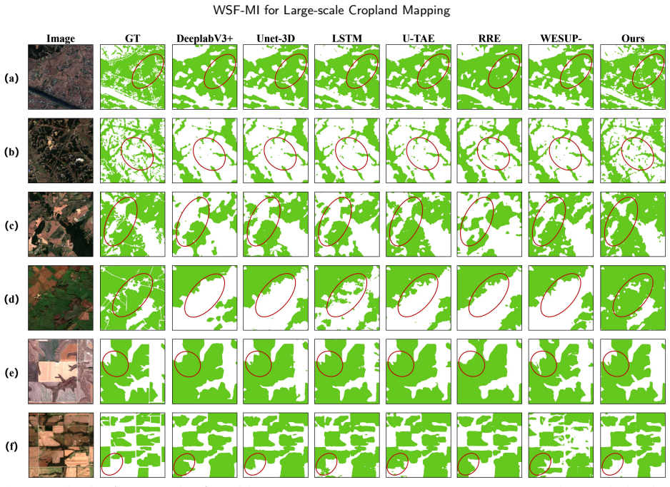
- It surpasses all six ATSG baselines on most metrics in all three areas, including the re-correct RRE method and the weakly supervised WESUP-LCP method.
- Whole-year SITS input is decisive: it improves average F1 by 3.47% to 5.22% over the best single-season composite, and t-SNE visualization shows the temporal features separate cropland better and tighten intra-class spread.
- Direct transfer from 2020 to 2021 without retraining fails to beat the best GLC products, but continue-training on the new year's unlabeled data still requires no manual labels and beats them by 1.82% to 2.87% in OA, mIoU, and F1.
- Under simulated cloud cover, the framework stays above the average of the three GLC products up to a 30% spatial mask and 66.67% temporal drop in Hunan, 10% and 33.33% in Southwest France, and 20% and 50% in Kansas.
Reading between the lines
- The label-accuracy versus label-ratio tradeoff visible in the paper's ablation table points to an adaptive consensus threshold: a two-product consensus can cover more area (up to 90.66%) but with lower accuracy, so an operational system could tune the number of agreeing products per region to maximize final map quality.
- Because the unsupervised regularizer is class-agnostic, the same consensus-plus-regularization recipe could be applied to any land-cover class, such as built-up, water, or forest, whenever multiple products provide a consensus mask, yielding a general no-label land-cover update mechanism.
- The direct-transfer failure implies the learned phenological features are year-specific; a promising extension the paper does not test is to feed both years' SITS into a single training run, or to fine-tune on a few hundred manually corrected pixels, which could lift transfer accuracy while keeping most of the label-free workflow.
Editorial analysis
A structured set of objections, weighed in public.
Referee Report
Summary. The paper proposes a weakly supervised framework (WSF-MI) for large-scale cropland mapping at 10 m resolution using dense Sentinel-2 satellite image time series (SITS). Training labels are generated by taking the consensus of three global land cover (GLC) products (ESA WorldCover, Esri Land Cover, Dynamic World); pixels where all three products agree are treated as high-quality labels for a supervised cross-entropy loss, while a regularizer based on visual similarity and spatial aggregation of the feature space is used as an unsupervised loss on both high- and low-quality samples. The U-TAE architecture is used as the multi-temporal segmentation network. Experiments are conducted in three large study areas (Hunan Province, Southwest France, Kansas), and the framework is reported to outperform the three GLC products and several automatic training sample generation (ATSG) baselines in terms of OA, mIoU, F1-scores, and related metrics. The paper also studies the effect of different GLC product combinations, temporal generalizability, the benefit of time-series information, and robustness to cloud/missing data. The source code is made publicly available.
Significance. If the reported results are reliable, the framework would offer a label-free way to improve over global cropland products at 10 m resolution, which is practically valuable for large-area agricultural monitoring. The idea of using consensus labels together with an unsupervised regularization term is well motivated and the temporal extension to exploit phenology is appropriate for the problem. The public code availability and the breadth of experiments (three distinct agro-ecosystems, ablation studies, robustness analysis) are positive features. However, the current evaluation protocol does not support the strong 'adaptability' claim made in the abstract, and the central comparison is partially circular because the supervised signal comes from the same GLC products used as baselines. The paper needs a substantially strengthened evaluation and clarification of a few technical issues before its conclusions can be accepted.
major comments (5)
- [§3.4 and §2.2] The validation sub-regions are spatially inside the training study area, and the paper argues in §3.4 that this overlap does not affect accuracy assessment because the training labels are pseudo-labels. This conflates label independence with spatial independence. The U-TAE is trained on 256x256 patches randomly sampled from the full study area, so the validation patches are very likely to appear in training; after 100 epochs the model may memorize their imagery and spatial layout, inflating all reported metrics (Tables 2-4). The claimed improvements over the best GLC products (e.g., Avg F1 +5.84% in Hunan, +0.51% in France, +1.40% in Kansas) are therefore not evidence of large-scale generalization. The authors should re-run the evaluation with validation patches excluded from training (including a buffer zone) or provide a cross-area validation (train on one study area, test on another) to support the 'strong adaptability' claim.
- [§5.2] The temporal direct-transfer (DT) result shows that a 2020-trained model does not beat the GLC products on 2021 data; only continued training (CT) with 2021 data yields improvements. The paper acknowledges this as a limitation, but it directly contradicts the abstract's claim of 'strong adaptability' and the general framing that the framework learns generic cropland phenology. At minimum, the conclusions should be tempered to reflect that adaptability is limited to within-year, within-area settings, and the DT result should be discussed as evidence of the model's sensitivity to temporal distribution shift rather than as a minor caveat.
- [Eq. (3)] The supervised loss is written as Loss_SL = - sum_i sum_j ( y(i,j) * log( M_high(i,j) * P(i,j) ) ). For any pixel where M_high(i,j)=0, the argument of the logarithm is 0, so the loss is undefined (log(0) is -infinity). The standard correct formulation is to mask the loss, e.g., Loss_SL = - sum_i sum_j M_high(i,j) * y(i,j) * log( P(i,j) ). As written, this core equation is mathematically invalid and needs to be corrected.
- [§4.3 and Table 5] The supervised training signal is derived from the consensus of exactly the three GLC products (ESA, Esri, Dynamic World) that are then used as comparison baselines in §4.3. This creates a partial circularity: the model cannot correct errors that are systematic across all three products, and its apparent improvement over each individual product may largely reflect a fusion effect. Table 5 indeed shows that the final prediction F1 closely tracks the consensus-label accuracy (e.g., Hunan DyWorld+Esri has the lowest label accuracy 75.33% and the lowest prediction F1 72.99%), confirming that the label source is the primary driver of performance. The paper should explicitly discuss this limitation and ideally design an experiment that isolates the contribution of the unsupervised loss, for example by training with only one GLC product as the label source and comparing to the consensus-based variant.
- [Tables 2-4] All accuracy metrics are point estimates from a single training run. Some of the claimed improvements are very small (e.g., Avg F1 +0.51% in France over Esri, +1.40% in Kansas over ESA), and these differences are within the typical run-to-run variance of deep learning training. The authors should report mean and standard deviation over at least three independent runs and, ideally, a significance test (e.g., paired test on patch-level errors) to support the claim that the framework 'achieved the best accuracy across most assessment metrics'.
minor comments (6)
- [§2.2] The product name 'ErisLandCover' is a typo and should be 'Esri Land Cover'.
- [§2.2] The sentence 'we labeled a total of 978,388 cropland fields' is ambiguous and, for manual visual interpretation, implausible as a field-level count; it is likely that these are pixels or object-based segments. Clarify the unit of labeling and how field-level annotations are converted to the pixel-level accuracy assessment.
- [Eq. (4)] The notation D_KL[Z(x_n), Z(x_n^s)] is not clearly defined. KL divergence is a measure between probability distributions, but Z is described as a fused intermediate feature map. Specify how the feature maps are converted to probability-like distributions (e.g., via softmax along the channel dimension) and over which axes the divergence is computed.
- [§5.2] The description 'randomly selected 1,000 samples of changed cropland' is unclear: does 'changed' refer to changes between 2020 and 2021, or changes within 2021? Also specify how these samples are distributed across the three study areas.
- [§4.1] No model-checkpoint selection criterion is stated. If the final model is chosen based on its performance on the validation set (which overlaps the training area), this would introduce another form of leakage. State the selection procedure explicitly.
- [§5.3] In the seasonal composite ablation, it is unclear whether the temporal encoding part is removed while still feeding a single composite image, or whether the input is reduced to one time step. Specify the exact input difference between the seasonal-composite runs and the full-SITS runs.
Circularity Check
No circularity: consensus-derived training labels are evaluated against independent manual validation, so the central accuracy claim is externally grounded.
full rationale
The paper's central derivation is a weakly supervised training framework whose supervised signal is the consensus of three GLC products (ESA, Esri, Dynamic World) and whose accuracy is then compared with those same products. This is a legitimate ATSG design, not a circular reduction, because the reported accuracies are computed against manually labeled validation datasets that are independent of the training labels. The model is not defined as the consensus of the products; it is a U-TAE trained with Eq. (3) supervised loss and Eq. (4) unsupervised regularization, and Table 3 shows it improves over every individual product, which would be impossible if the prediction were simply a re-expression of the inputs. No parameter is fitted to the validation set, and no result is renamed from a fitted input. There are no load-bearing self-citations: the cited unsupervised-learning assumptions (Hua et al. 2021; Sabokrou et al. 2019) are external prior work, and U-TAE is cited as a standard architecture. One passage, Section 3.4, asserts that 'The overlap between the training and validation sets will not affect the accuracy assessment process' because the training labels are pseudo-labels. This is a legitimate methodological concern about spatial data leakage and generalization claims, but it is not a circularity: the validation labels are manually created, so the evaluation does not reduce to the training signal. Accordingly, the circularity score is 0.
Assumptions & free parameters
free parameters (3)
- alpha =
not reported
- beta =
not reported
- gamma =
not reported
assumptions (5)
- domain assumption Full agreement among ESA, Esri, and Dynamic World implies a correct cropland label for that pixel.
- domain assumption Visually similar image patches tend to have the same semantic class.
- domain assumption Land cover is spatially continuous and aggregated, so neighboring similar pixels share a class.
- domain assumption Monthly composites made by averaging available images preserve the phenological signal needed to separate cropland.
- domain assumption Manually interpreted validation labels are accurate enough to assess the maps.
Cite this review
Pith. "Pith review of Weakly Supervised Framework Considering Multi-temporal Information for Large-scale Cropland Mapping with Satellite Imagery." pith.science (2026). https://pith.science/paper/5UZWWK2P
@misc{pith2026241118475,
  author       = {Pith},
  title        = {Pith review of: Weakly Supervised Framework Considering Multi-temporal Information for Large-scale Cropland Mapping with Satellite Imagery},
  year         = {2026},
  howpublished = {\url{https://pith.science/paper/5UZWWK2P}},
  note         = {Machine review of arXiv:2411.18475}
}
read the original abstract
Accurately mapping large-scale cropland is crucial for agricultural production management and planning. Currently, the combination of remote sensing data and deep learning techniques has shown outstanding performance in cropland mapping. However, those approaches require massive precise labels, which are labor-intensive. To reduce the label cost, this study presented a weakly supervised framework considering multi-temporal information for large-scale cropland mapping. Specifically, we extract high-quality labels according to their consistency among global land cover (GLC) products to construct the supervised learning signal. On the one hand, to alleviate the overfitting problem caused by the model's over-trust of remaining errors in high-quality labels, we encode the similarity/aggregation of cropland in the visual/spatial domain to construct the unsupervised learning signal, and take it as the regularization term to constrain the supervised part. On the other hand, to sufficiently leverage the plentiful information in the samples without high-quality labels, we also incorporate the unsupervised learning signal in these samples, enriching the diversity of the feature space. After that, to capture the phenological features of croplands, we introduce dense satellite image time series (SITS) to extend the proposed framework in the temporal dimension. We also visualized the high dimensional phenological features to uncover how multi-temporal information benefits cropland extraction, and assessed the method's robustness under conditions of data scarcity. The proposed framework has been experimentally validated for strong adaptability across three study areas (Hunan Province, Southeast France, and Kansas) in large-scale cropland mapping, and the internal mechanism and temporal generalizability are also investigated.
Figures


Figures from the paper (12 more)




Reference graph
Works this paper leans on
-
[5]
Near real-time agriculture monitoring atnationalscaleatparcelresolution:PerformanceassessmentoftheSen2-Agriautomatedsysteminvariouscroppingsystemsaroundtheworld. Remote Sensing of Environment 221, 551–568.https://linkinghub.elsevier.com/retrieve/pii/S0034425718305145. Deng,P.,Xu,K.,Huang,H.,2021. Whencnnsmeetvisiontransformer:Ajointframeworkforremotesensi...
work page 2021
-
[7]
Garnot,V.S.F.,Landrieu,L.,2020
MCD12Q1 MODIS/Terra+Aqua Land Cover Type Yearly L3 Global 500m SIN Grid V006.https: //lpdaac.usgs.gov/products/mcd12q1v006/. Garnot,V.S.F.,Landrieu,L.,2020. LightweightTemporalSelf-attentionforClassifyingSatelliteImagesTimeSeries,in:Lemaire,V.,Malinowski, S.,Bagnall,A.,Guyet,T.,Tavenard,R.,Ifrim,G.(Eds.),AdvancedAnalyticsandLearningonTemporalData.Springer...
-
[10]
Agricultural remote sensing big data: Management and applications. Journal of Integrative Agriculture 17, 1915–1931.https://linkinghub.elsevier.com/retrieve/pii/S2095311917618598. Jiang, B.,
work page 1915
-
[13]
Cropland data fusion and correction using spatial analysis techniques and the Google Earth Engine. GIScience & Remote Sensing 57, 1026–1045.https://www.tandfonline.com/doi/full/10.1080/15481603.2020.1841489. Liu, Y., Wu, Y., Chen, Z., Huang, M., Du, W., Chen, N., Xiao, C.,
-
[14]
A Novel Impervious Surface Extraction Method Based on Automatically Generating Training Samples From Multisource Remote Sensing Products: A Case Study of Wuhan City, China. IEEE J. Sel. Top. Appl. Earth Observations Remote Sensing 15, 6766–6780.https://ieeexplore.ieee.org/document/9854083/. Naboureh, A., Li, A., Bian, J., Lei, G.,
-
[15]
National Scale Land Cover Classification Using the Semiautomatic High-Quality Reference Sample Generation (HRSG) Method and an Adaptive Supervised Classification Scheme. IEEE J. Sel. Top. Appl. Earth Observations Remote Sensing 16, 1858–1870. https://ieeexplore.ieee.org/document/10035401/. Nanni, L., Ghidoni, S., Brahnam, S.,
-
[16]
Boundary Delineation of Agricultural Fields in Multitemporal Satellite Imagery. IEEE J. Sel. Top. Appl. Earth Observations Remote Sensing 12, 237–251.https://ieeexplore.ieee.org/document/8584043/. Oliphant,A.J.,Thenkabail,P.S.,Teluguntla,P.,Xiong,J.,Gumma,M.K.,Congalton,R.G.,Yadav,K.,2019. MappingcroplandextentofSoutheast and Northeast Asia using multi-ye...
-
[17]
75–82.https://api.semanticscholar.org/CorpusID:198180478
Semantic segmentation of crop type in africa: A novel dataset and analysis of deep learning methods, in: CVPR Workshops, pp. 75–82.https://api.semanticscholar.org/CorpusID:198180478. Sabokrou,M.,Khalooei,M.,Adeli,E.,2019. Self-SupervisedRepresentationLearningviaNeighborhood-RelationalEncoding,in:2019IEEECVF Int. Conf. Comput. Vis. ICCV, IEEE, Seoul, Korea...
Show all 26 references
-
[18]
InternationalJournalofRemoteSensing40,593–614
Using long short-term memory recurrent neural network in land cover classification on Landsat and Cropland data layertimeseries. InternationalJournalofRemoteSensing40,593–614. https://www.tandfonline.com/doi/full/10.1080/01431161. 2018.1516313. Sykas, D., Sdraka, M., Zografaki...
-
[19]
A Sentinel-2 Multiyear, Multicountry Benchmark Dataset for Crop Classification and Segmentation With Deep Learning. IEEE J. Sel. Top. Appl. Earth Observations Remote Sensing 15, 3323–3339.https://ieeexplore. ieee.org/document/9749916/. Wagner, M.P., Oppelt, N.,
-
[20]
Remote Sensing 12, 1205.https://www.mdpi.com/2072-4292/12/7/1205
Extracting Agricultural Fields from Remote Sensing Imagery Using Graph-Based Growing Contours. Remote Sensing 12, 1205.https://www.mdpi.com/2072-4292/12/7/1205. Wang, Y., Wang, H., Shen, Y., Fei, J., Li, W., Jin, G., Wu, L., Zhao, R., Le, X.,
-
[21]
Semi-Supervised Semantic Segmentation Using Unreliable Pseudo-Labels, in: 2022 IEEECVF Conf. Comput. Vis. Pattern Recognit. CVPR, IEEE, New Orleans, LA, USA. pp. 4238–4247. https://ieeexplore.ieee.org/document/9879387/. Weiss, M., Jacob, F., Duveiller, G.,
2022
-
[22]
Remote Sensing 10, 1623.http://www.mdpi.com/ 2072-4292/10/10/1623
A National Assessment of Wetland Status and Trends for Canada’s Forested Ecosystems Using 33 Years of Earth Observation Satellite Data. Remote Sensing 10, 1623.http://www.mdpi.com/ 2072-4292/10/10/1623. Wulder,M.A.,Dechka,J.A.,Gillis,M.A.,Luther,J.E.,Hall,R.J.,Beaudoin,A.,Fran...
2003 doi
-
[24]
International Journal of Remote Sensing 34, 5851–5867.https://www.tandfonline.com/doi/full/10
Improving 30 m global land-cover map FROM-GLC with time series MODIS and auxiliary data sets: A segmentation-based approach. International Journal of Remote Sensing 34, 5851–5867.https://www.tandfonline.com/doi/full/10. 1080/01431161.2013.798055. Yue,A.,Zhang,C.,Yang,J.,Su,W.,...
-
[25]
IEEETrans.Geosci.RemoteSensing61,1–16
A Novel Knowledge-Driven Automated Solution for High-ResolutionCroplandExtractionbyCross-ScaleSampleTransfer. IEEETrans.Geosci.RemoteSensing61,1–16. https://ieeexplore. ieee.org/document/10197441/. Zhong, L., Hu, L., Zhou, H.,
-
[26]
IEEE Geosci
Deep Learning in Remote Sensing: A Comprehensive Review and List of Resources. IEEE Geosci. Remote Sens. Mag. 5, 8–36. doi:10.1109/MGRS.2017.2762307. Zhu,Z.,Gallant,A.L.,Woodcock,C.E.,Pengra,B.,Olofsson,P.,Loveland,T.R.,Jin,S.,Dahal,D.,Yang,L.,Auch,R.F.,2016. Optimizingselecti...
2017
-
[2010]
FareGarnot,V.S.,Landrieu,L.,2021
World programme for the census of agriculture. FareGarnot,V.S.,Landrieu,L.,2021. PanopticSegmentationofSatelliteImageTimeSerieswithConvolutionalTemporalAttentionNetworks,in: 2021IEEECVFInt.Conf.Comput.Vis.ICCV,IEEE,Montreal,QC,Canada.pp.4852–4861. https://ieeexplore.ieee.org/d...
2021
-
[2013]
International Journal of Remote Sensing 34, 2607–2654
Finer resolution observation Yuze.W: Preprint submitted to Elsevier Page 23 of 25 WSF-MI for Large-scale Cropland Mapping and monitoring of global land cover: First mapping results with Landsat TM and ETM+ data. International Journal of Remote Sensing 34, 2607–2654. https://ww...
-
[2015]
GeoJournal 80, 1–13.http: //link.springer.com/10.1007/s10708-014-9537-y
Geospatial analysis requires a different way of thinking: The problem of spatial heterogeneity. GeoJournal 80, 1–13.http: //link.springer.com/10.1007/s10708-014-9537-y. Karra,K.,Kontgis,C.,Statman-Weil,Z.,Mazzariello,J.C.,Mathis,M.,Brumby,S.P.,2021a. Globallanduse/landcoverwit...
-
[2016]
Big Data for Remote Sensing: Challenges and Opportunities. Proc. IEEE 104, 2207–2219. https://ieeexplore.ieee.org/document/7565634/. Coluzzi, R., Imbrenda, V., Lanfredi, M., Simoniello, T.,
-
[2017]
InternationalJournalofRemoteSensing38,4459–4480
Monitoring cropland changes along the Nile River in Egypt over past three decades(1984–2015)usingremotesensing. InternationalJournalofRemoteSensing38,4459–4480. https://www.tandfonline.com/doi/ full/10.1080/01431161.2017.1323285. Yin, J., Dong, J., Hamm, N.A., Li, Z., Wang, J....
1984
-
[2018]
volume 11211, pp
Encoder-Decoder with Atrous Separable Convolution for Semantic Image Segmentation,in:Ferrari,V.,Hebert,M.,Sminchisescu,C.,Weiss,Y.(Eds.),ComputerVision–ECCV2018.SpringerInternationalPublishing, Cham. volume 11211, pp. 833–851.https://link.springer.com/10.1007/978-3-030-01234-2...
-
[2019]
https://cds.climate.copernicus.eu/doi/10.24381/cds.006f2c9a
Land cover classification gridded maps from 1992 to present derived from satellite observations. https://cds.climate.copernicus.eu/doi/10.24381/cds.006f2c9a. Defourny, P., Bontemps, S., Bellemans, N., Cara, C., Dedieu, G., Guzzonato, E., Hagolle, O., Inglada, J., Nicola, L., R...
1992 doi
-
[2020]
Google Earth Engine Cloud Computing Platform for Remote Sensing Big Data Applications: A Comprehensive Review. IEEE J. Sel. Top. Appl. Earth Observations Remote Sensing 13, 5326–5350.https://ieeexplore.ieee.org/ document/9184118/. Belgiu, M., Csillik, O.,
-
[2022]
Remote Sensing of Environment 268, 112780
Land cover classification in an era of big and open data: Optimizing localized implementation and training data selection to improve mapping outcomes. Remote Sensing of Environment 268, 112780. https:// linkinghub.elsevier.com/retrieve/pii/S0034425721005009. Hua,Y.,Marcos,D.,M...
2021
-
[2023]
Remote Sensing of Environment 294, 113623
Development of a 10-m resolution maize and soybean map over china: Matching satellite-based crop classification with sample-based area estimation. Remote Sensing of Environment 294, 113623. Li,J.,Huang,X.,Gong,J.,2019.Deepneuralnetworkforremote-sensingimageinterpretation:Statu...
2019
Reviewed August 12, 2026 · model on record in the stance chip above.
Discussion (0). Continue with ORCID to comment.