REVIEW 4 major objections 6 minor 25 references
A Learn-to-Optimize Approach for Coordinate-Wise Step Sizes for Quasi-Newton Methods
T0 review · 4 major / 6 minor · reviewed 2026-08-12 · deepseek-v4-flash
Pith's one-line read A learned LSTM supplies coordinate-wise step sizes for BFGS, up to 4× faster than line search and hypergradient descent, while respecting sufficient convergence conditions.
desk verdict Plausible L2O method with a broken theory-to-implementation bridge: the (0,2) step-size clamp is a relaxation of the theorem's bound, not a corollary, so the central guarantee claim needs rework. read the letter →
The pith
A machine-rendered reading of the paper's core claim, the machinery that carries it, and where it could break.
The reading
What carries the argument
The load-bearing object is the diagonal coordinate-wise step-size matrix $P_k=\mathrm{diag}(2\sigma(p_k))$, produced by an LSTM plus an MLP and clamped so each entry lies in $(0,2)$. The theoretical support is a safe operating region defined by three sufficient conditions: the norm conditions of Theorem 1, the entrywise bound $0<p_{k,i}\le 2\gamma/L$ where $\gamma$ is the smallest eigenvalue of the approximate Hessian $B_k$, and the asymptotic requirement $P_k\to I$ from Theorem 3. The training objective $f(x_{k+1})+\lambda\|P_k-I\|_F^2$ operationalizes these conditions: the first term drives fast descent, while the regularization encourages the identity limit that preserves BFGS's superlinear convergence.
What would settle it
Take a strongly convex quadratic whose Hessian has a very small eigenvalue $\gamma$ relative to its largest eigenvalue $L$. Run the paper's BFGS-L2O method from a start point far from the optimum and record $\|x_{k+1}-x^*\|$; a single iteration where $\max_i p_{k,i} > 2\gamma/L$ and the distance to the optimum increases would violate Theorem 2 and falsify the claim that clamping to $(0,2)$ respects the derived conditions.
Extended reading notes
Core claim
The paper's central claim is that coordinate-wise step sizes for BFGS can be generated by a neural network and still respect the convergence guarantees of quasi-Newton methods. Theoretically, it proves three sufficient conditions: a norm bound on $P_k$ and a related bound on $P_k^{-1}$ force the gradient norms to vanish (Theorem 1); for convex $L$-smooth objectives with uniformly lower-bounded Hessian approximations, entrywise bounds $0<p_{k,i}\le 2\gamma/L$ make each step monotonically closer to the minimizer (Theorem 2); and if $P_k\to I$ along a convergent trajectory, BFGS keeps its superlinear rate (Theorem 3). On the algorithmic side, an LSTM shared across coordinates maps $(x_k,\nabla f(x_k),B_k^{-1}\nabla f(x_k))$ to a diagonal $P_k=\mathrm{diag}(2\sigma(p_k))$, trained to minimize the next objective value plus a regularization $\lambda\|P_k-I\|_F^2$ that pushes the step sizes toward identity near the optimum. The paper reports that this trained policy converges up to 4× faster than backtracking line search and hypergradient descent across the tested problems.
Load-bearing premise
The load-bearing premise is that bounding every coordinate-wise step size to the interval $(0,2)$ automatically satisfies the paper's sufficient conditions; that reduction identifies $2\gamma/L$ with $2$, which is safe only when the smallest curvature $\gamma$ of the Hessian approximation is comparable to the smoothness constant $L$, not when $\gamma\ll L$.
Editorial extensions
If this is right
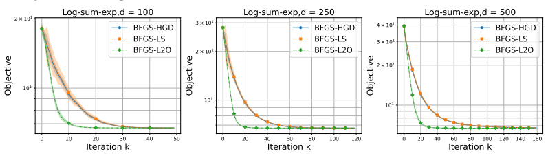
- On the tested least squares and log-sum-exp problems, BFGS with learned coordinate-wise step sizes reaches the target objective in roughly 25% to 75% fewer iterations than line search; for log-sum-exp the speedup grows from 2× at dimension 100 to 4× at dimension 500.
- The same shared LSTM handles different problem dimensions without adding parameters, so the method scales to higher-dimensional optimization tasks.
- Near the optimum the regularization term pushes $P_k$ toward the identity, so the learned step sizes hand control back to the unmodified BFGS update and preserve its superlinear convergence.
- Hypergradient descent on the step-size matrix gives only marginal gains after the first few BFGS iterations, and can be unstable on neural network training, whereas the learned policy is reported to be more stable.
Reading between the lines
- The practical simplification that clamps step sizes to $(0,2)$ is only guaranteed by Theorem 2 when $2\gamma/L\ge 2$; on ill-conditioned objectives with $\gamma\ll L$, entries near 2 could fall outside the proven safe region, so estimating $\gamma$ locally and shrinking the upper bound would make the guarantee airtight.
- Because the LSTM is trained on a distribution of random problem instances, its speedup is likely tied to shared structure in that distribution; on objectives whose geometry differs strongly from the training set, the learned policy may degrade to or below the line-search baseline.
- The frequent outer-loop updates after every inner iteration are a deliberate response to the dual role of step sizes in BFGS, since a step affects both the iterate and the Hessian approximation; testing longer unrolls or a surrogate that predicts curvature quality could reveal the trade-off between responsiveness and meta-training stability.
Editorial analysis
A structured set of objections, weighed in public.
Referee Report
Summary. The paper proposes a learn-to-optimize (L2O) method that uses an LSTM/MLP to generate coordinate-wise step-size matrices for BFGS updates. It first derives sufficient conditions for coordinate-wise step sizes in BFGS (Theorems 1–3) and then argues that the proposed architecture, which outputs step sizes in (0,2) via a scaled sigmoid, inherently respects these conditions. The method is evaluated on least squares, logistic regression, log-sum-exp problems, and a simple CNN training task, reporting up to 4x faster convergence in iterations compared to backtracking line search and hypergradient descent. The paper includes proofs in an appendix and a limitations section.
Significance. If the theoretical-to-implementation bridge were sound, the paper would be a useful contribution to the under-explored area of step-size tuning in quasi-Newton methods, combining a theoretical sufficient-condition analysis with a data-driven L2O policy. The empirical study is reasonably broad, covers several problem classes with increasing dimension, and reports consistent iteration-count speedups. The paper also provides complete proofs of the stated theorems and uses a standard meta-learning train/test split, which avoids circularity in the experimental protocol. However, the central claim that the implemented constraint (0,2) 'inherently respects' the derived sufficient conditions is not correct, and this affects the main narrative of guaranteed stability and convergence. The practical value of the empirical speedups is also limited by the absence of wall-clock time measurements and code. With a corrected theoretical justification or an explicitly weakened claim, the empirical contribution could still stand, but the current form overstates the theoretical grounding.
major comments (4)
- [Section 3.3, Theorem 2 and its remark; Section 4] The implementation constraint P_k = diag(2σ(p_k)) with entries in (0,2) does not imply the sufficient condition 0 < p_{k,i} ≤ 2γ/L of Theorem 2. The remark that the upper bound 2γ/L 'simplifies to 2' is mathematically incorrect: since γ ≤ L, the ratio 2γ/L is at most 2, and it can be arbitrarily close to 0 when the Hessian is ill-conditioned. Therefore, allowing p_{k,i} up to 2 admits step sizes that violate Theorem 2 whenever γ < L. The same problem affects Theorem 1, whose upper bound ∥P_k∥_2 ≤ α/(L∥B_k^{-1}\|_2) is strictly less than 2 because ∥B_k^{-1}\|_2 ≥ 1/∥B_k\|_2 and ∥B_k\|_2 ≤ L, making the bound no larger than α < 2. Consequently, the abstract and Section 4 claim that the method 'inherently respects the derived theoretical guarantees' is unsupported. The paper should either enforce the actual problem-dependent bound (for instance, by estimating γ and L) or explicitly present the (0,2) constraint as a heuristic simplification that is motivated by, but not guaranteed to satisfy, the theorems.
- [Appendix D and Section 4] The 'practical and robust simplification' described in Section 4 runs in the wrong direction: the theoretical safe region is a subset of (0,2), while the implementation permits all of (0,2), including values that can violate the sufficient conditions. Appendix D's limitation statement only notes that the constraint might preclude faster strategies outside the bounds; it does not acknowledge that the constraint can also admit unsafe step sizes. Because the claimed stability and convergence guarantees hinge on the step sizes satisfying the theorems, this omission must be corrected, either by changing the architecture or by explicitly stating that the guarantees do not apply to the implemented algorithm.
- [Section 5 (Experiments)] All reported speedups are in iteration counts. The BFGS-L2O method incurs additional per-iteration cost from the LSTM and MLP forward passes, while the backtracking line search baseline also requires function evaluations. Without wall-clock time measurements, the headline claim of 'up to 4× faster convergence' is not established as an actual runtime speedup. Please include wall-clock comparisons or explicitly qualify the speedup as iteration-wise convergence.
- [Appendix B and code availability] The paper does not provide code, and the description of the L2O model is incomplete: the LSTM hidden size, MLP architecture, regularization coefficient λ, the number of inner-loop iterations K, and the exact training details are not specified beyond 200 Adam updates with batch size 64. Since the L2O model is the central methodological contribution, this level of detail is insufficient to reproduce or verify the empirical results. Releasing code and reporting the full hyperparameter settings would substantially strengthen the paper.
minor comments (6)
- [Section 2] The phrase 'In this chapter' should be 'In this section' for consistency with the rest of the paper.
- [Section 3.1 and Appendix C] The formula P_k = α*_k I − (1/LR) v_k B^{-1}_k ∇f(x_k) appears dimensionally inconsistent: v_k is defined as a diagonal matrix, so v_k B^{-1}_k ∇f(x_k) is a vector, which cannot be subtracted from a matrix. Please clarify the intended construction, presumably involving diag(v_k ⊙ B^{-1}_k ∇f(x_k)) or a similar outer-product form.
- [Appendix B.3] The sentence 'Following the setup in [16] (from your main text)' contains a leftover template instruction and should be removed.
- [Appendix A.1, proof of Theorem 1] The second inequality in the proof uses a condition on λ_max(P_k), but the theorem statement gives a condition on ∥P^{-1}\|_2, which is equivalent to a lower bound on λ_min(P_k). Please reconcile this mismatch.
- [Figure 1] Unlike Figure 4, Figure 1 shows a single curve without variance or error bars; adding multiple seeds would improve the reliability of the reported improvement.
- [Theorem 2 proof] In the proof of Theorem 2, T_k is not symmetric, so statements about 'the eigenvalue of T_k' should be phrased in terms of spectral radius or singular values rather than eigenvalues without qualification.
Circularity Check
No significant circularity: the (0,2) bound is an invalid simplification, not a circular fit; only a minor, non-load-bearing self-citation.
full rationale
The paper's derivation chain is largely self-contained. Theorems 1-3 are proved in Appendix A from standard assumptions (L-smoothness, gamma I <= B_k, well-conditioned B_k) and do not use the experimental data; the LSTM is trained on a random training distribution and evaluated on held-out samples from the same generator, which is ordinary meta-learning and not a fitted-parameter prediction. The one overlapping-author citation ([23]) appears only to justify that assumptions are 'common' and to describe unrolling choices; none of the theorems or the sigmoid architecture depends on it, so it is not load-bearing. The real weakness is the paper's remark that the Theorem 2 bound 2 gamma / L 'simplifies to 2': since gamma <= L gives 2 gamma / L <= 2, enforcing p in (0,2) is weaker than the sufficient condition p <= 2 gamma / L. This is an unsupported inference that undercuts the claim of 'inherently respecting' the theorems, but it is a logical/correctness gap, not a circularity--it does not equate a prediction to a fit or a theorem to its input. Hence the circularity score is low.
Assumptions & free parameters
free parameters (3)
- LSTM/MLP weights (φ_LSTM, φ_MLP) =
trained, not reported
- Output scale 2 in P=diag(2σ(p)) =
2
- Regularization coefficient λ and inner-loop iterations K =
not reported
assumptions (5)
- domain assumption Objective f is L-smooth (Assumption 1)
- domain assumption f is twice differentiable on an open convex set and the Hessian is continuous and nonsingular at the minimizer (Assumption 2)
- domain assumption BFGS Hessian approximations B_k are positive definite with cond(B_k) ≤ M and update directions are bounded (Assumptions 3 and 4)
- standard math Dennis-More style BFGS superlinear convergence, ||B_k - ∇²f(x*)|| / ||x_{k+1}-x_k|| tends to 0 (Theorem 3.4 of [10])
- ad hoc to paper Eigenvalues of B_k lie within [γ,L] and therefore 2γ/L simplifies to 2
Cite this review
Pith. "Pith review of A Learn-to-Optimize Approach for Coordinate-Wise Step Sizes for Quasi-Newton Methods." pith.science (2026). https://pith.science/paper/PE4PGQ53
@misc{pith2026241200059,
  author       = {Pith},
  title        = {Pith review of: A Learn-to-Optimize Approach for Coordinate-Wise Step Sizes for Quasi-Newton Methods},
  year         = {2026},
  howpublished = {\url{https://pith.science/paper/PE4PGQ53}},
  note         = {Machine review of arXiv:2412.00059}
}
abstract
Tuning step sizes is crucial for the stability and efficiency of optimization algorithms. While adaptive coordinate-wise step sizes have been shown to outperform scalar step size in first-order methods, their use in second-order methods is still under-explored and more challenging. Current approaches, including hypergradient descent and cutting plane methods, offer limited improvements or encounter difficulties in second-order contexts. To address these limitations, we first conduct a theoretical analysis within the Broyden-Fletcher-Goldfarb-Shanno (BFGS) framework, a prominent quasi-Newton method, and derive sufficient conditions for coordinate-wise step sizes that ensure convergence and stability. Building on this theoretical foundation, we introduce a novel learn-to-optimize (L2O) method that employs LSTM-based networks to learn optimal step sizes by leveraging insights from past optimization trajectories, while inherently respecting the derived theoretical guarantees. Extensive experiments demonstrate that our approach achieves substantial improvements over scalar step size methods and hypergradient descent-based method, offering up to 4$\times$ faster convergence across diverse optimization tasks.
Figures

Reference graph
Works this paper leans on
-
[15]
Searching for Optimal Per-Coordinate Step-Sizes with Multidimensional Backtracking
Frederik Kunstner, Victor Sanches Portella, Mark Schmidt, and Nicholas Harvey. Searching for Optimal Per-Coordinate Step-Sizes with Multidimensional Backtracking. In NeurIPS, volume 36, pages 2725–2767, 2023
work page 2023
-
[1]
Step-size Adaptation Using Exponentiated Gradient Updates
Ehsan Amid, Rohan Anil, Christopher Fifty, and Manfred K Warmuth. Step-Size Adaptation Using Exponentiated Gradient Updates. arXiv preprint arXiv:2202.00145, 2022
work page Pith review arXiv 2022
-
[2]
Learning to Learn by Gradient Descent by Gradient Descent
Marcin Andrychowicz, Misha Denil, Sergio Gomez, Matthew W Hoffman, David Pfau, Tom Schaul, Brendan Shillingford, and Nando De Freitas. Learning to Learn by Gradient Descent by Gradient Descent. In NeurIPS, volume 29, 2016
work page 2016
-
[3]
Minimization of Functions Having Lipschitz Continuous First Partial Derivatives
Larry Armijo. Minimization of Functions Having Lipschitz Continuous First Partial Derivatives. Pacific Journal of Mathematics, 16(1):1–3, 1966
work page 1966
-
[4]
An Introduction to Numerical Analysis
Kendall Atkinson. An Introduction to Numerical Analysis. John wiley & sons, 1991
work page 1991
-
[5]
First-Order Methods in Optimization
Amir Beck. First-Order Methods in Optimization. SIAM, 2017
2017
-
[6]
Stephen Boyd and Lieven Vandenberghe. Convex Optimization. Cambridge university press, 2004
work page 2004
-
[7]
A Class of Methods for Solving Nonlinear Simultaneous Equations
Charles G Broyden. A Class of Methods for Solving Nonlinear Simultaneous Equations. Mathematics of Computation, 19(92):577–593, 1965
work page 1965
Show all 25 references
-
[8]
Quasi-Newton Methods and Their Application to Function Minimisation.Mathematics of Computation, 21(99):368–381, 1967
Charles G Broyden. Quasi-Newton Methods and Their Application to Function Minimisation.Mathematics of Computation, 21(99):368–381, 1967
1967
-
[9]
Convergence of Quasi-Newton Matrices Generated by the Symmetric Rank One Update
Andrew R Conn, Nicholas IM Gould, and Ph L Toint. Convergence of Quasi-Newton Matrices Generated by the Symmetric Rank One Update. Mathematical Programming, 50(1):177–195, 1991
1991
-
[10]
A Characterization of Superlinear Convergence and Its Application to Quasi-Newton Methods
John E Dennis and Jorge J Moré. A Characterization of Superlinear Convergence and Its Application to Quasi-Newton Methods. Mathematics of Computation, 28(126):549–560, 1974
1974
-
[11]
Quasi-Newton Methods, Motivation and Theory
John E Dennis, Jr and Jorge J Moré. Quasi-Newton Methods, Motivation and Theory. SIAM Review, 19(1):46–89, 1977
1977
-
[12]
Adaptive Subgradient Methods for Online Learning and Stochastic Optimization
John Duchi, Elad Hazan, and Yoram Singer. Adaptive Subgradient Methods for Online Learning and Stochastic Optimization. Journal of Machine Learning Research, 12(7), 2011
2011
-
[13]
Neural Networks for Machine Learning, Lecture 6, 2012
Geoffrey Hinton. Neural Networks for Machine Learning, Lecture 6, 2012
2012
-
[14]
Adam: A Method for Stochastic Optimization
Diederik P Kingma. Adam: A Method for Stochastic Optimization. In ICLR, 2015
2015
-
[16]
Towards Constituting Mathe- matical Structures for Learning to Optimize
Jialin Liu, Xiaohan Chen, Zhangyang Wang, Wotao Yin, and HanQin Cai. Towards Constituting Mathe- matical Structures for Learning to Optimize. In ICML, pages 21426–21449. PMLR, 2023
2023
-
[17]
Learning Gradient Descent: Better Generalization and Longer Horizons
Kaifeng Lv, Shunhua Jiang, and Jian Li. Learning Gradient Descent: Better Generalization and Longer Horizons. In ICML, pages 2247–2255. PMLR, 2017
2017
-
[18]
Gradient-Based Hyperparameter Optimization through Reversible Learning
Dougal Maclaurin, David Duvenaud, and Ryan Adams. Gradient-Based Hyperparameter Optimization through Reversible Learning. In ICML, pages 2113–2122, 2015
2015
-
[19]
Speed Learning on the Fly
Pierre-Yves Massé and Yann Ollivier. Speed Learning on the Fly. arXiv preprint arXiv:1511.02540, 2015
2015 arXiv
-
[20]
Fast Exact Multiplication by the Hessian
Barak A Pearlmutter. Fast Exact Multiplication by the Hessian. Neural Computation, 6(1):147–160, 1994
1994
-
[21]
Greedy Quasi-Newton Methods with Explicit Superlinear Conver- gence
Anton Rodomanov and Yurii Nesterov. Greedy Quasi-Newton Methods with Explicit Superlinear Conver- gence. SIAM Journal on Optimization, 31(1):785–811, 2021
2021
-
[22]
Large-Scale Convex Optimization: Algorithms & Analyses via Monotone Operators
Ernest K Ryu and Wotao Yin. Large-Scale Convex Optimization: Algorithms & Analyses via Monotone Operators. Cambridge University Press, 2022
2022
-
[23]
Towards Robust Learning to Optimize with Theoretical Guarantees
Qingyu Song, Wei Lin, Juncheng Wang, and Hong Xu. Towards Robust Learning to Optimize with Theoretical Guarantees. In CVPR, pages 27498–27506, 2024
2024
-
[24]
Stochastic Quasi-Newton with Adaptive Step Lengths for Large-Scale Problems
Adrian Wills and Thomas Schön. Stochastic Quasi-Newton with Adaptive Step Lengths for Large-Scale Problems. arXiv preprint arXiv:1802.04310, 2018
2018 arXiv
-
[25]
safe operating region
Stephen J Wright. Numerical Optimization, 2006. 10 A Proofs A.1 Proof of Theorem 1 Proof. Consider a quadratic function Q(x) =f (y) +∇f (y)⊤(x − y) +α 2 (x − y)⊤BkP −1 k (x − y). Basically, we use this quadratic function as a local approximation of f (x) around y, and we think...
2006
Reviewed August 12, 2026 · model on record in the stance chip above.
Discussion (0). Continue with ORCID to comment.