REVIEW 3 major objections 4 minor 52 references
Messenger size optimality in cellular communications
T0 review · 3 major / 4 minor · reviewed 2026-08-12 · deepseek-v4-flash
Pith's one-line read A physical tradeoff among synthesis, diffusion, degradation, and binding predicts optimal messenger protein sizes, explaining why chemokines cluster in a narrow mass range.
desk verdict A clean simulation of a size-dependent messenger tradeoff, but the central optimality is built in by a hand-picked degradation scaling and an assumed information-per-length term, so the chemokine claim is not yet earned. read the letter →
The pith
A machine-rendered reading of the paper's core claim, the machinery that carries it, and where it could break.
The reading
What carries the argument
The argument is carried by a discrete-time stochastic simulation of synthesis, diffusion, degradation, and binding whose input terms scale with protein length $L_p$: synthesis energy cost $\Delta E_s$ grows with $L_p$; the diffusion coefficient is $D \propto L_p^{-0.33}$; the degradation probability is $p_{\mathrm{deg}} = V_{\max}/(K_M + P_t)$ with $K_M = (L_p/2)^{\delta}$ and $\delta \approx 2$; and the binding probability is $p_{\mathrm{on}} = (L_p/2)^{-\beta}$ with $\beta = 3/2$. The steep degradation-size relation is the balancing term that lets larger proteins remain competitive despite slower diffusion, costlier synthesis, and weaker binding. Performance is scored by the ratios $\eta_E = L_p B / E$, $\eta_T = L_p B / T$, and $\eta_N = L_p B / N$, treating each bound protein as carrying $L_p$ bits of information.
What would settle it
Measure the extracellular degradation half-life of a size series of secreted proteins (for example 2, 4, 8, 16, and 32 kDa) in the same medium. If the half-life does not grow about as the square of protein length over that range, the degradation term that creates the optimal sizes in the model is absent, and rerunning the simulation with measured degradation rates should erase the predicted efficiency peaks.
Extended reading notes
Core claim
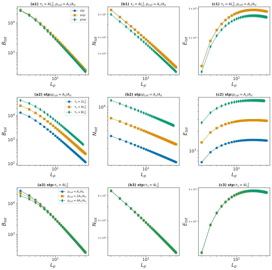
The central claim is that optimal messenger sizes emerge from a competition among processes that favor small proteins and one that favors large proteins. Small proteins are cheap to synthesize, diffuse quickly, and bind readily; large proteins survive longer in the extracellular space because the degradation probability is taken to fall steeply with size. Across three signal shapes (step, exponential, and power-law), the simulation produces efficiency maxima: total information per time and per generated protein peak around $L_p<10$, while information per energy at the moment of maximum receptor occupancy and the other peak-occupancy efficiencies peak at $L_p>10$, with the optimum shifting upward as signal duration or collision probability increases. The authors conclude that the narrow molecular-mass window of natural secreted messengers reflects this size–cost tradeoff.
Load-bearing premise
The result depends on the assumption that extracellular degradation becomes much slower for larger proteins, steeply enough (roughly as protein length squared) to compensate for the disadvantages of larger proteins in synthesis cost, diffusion, and binding; if real degradation does not scale this way, the predicted optimal sizes disappear.
Editorial extensions
If this is right
- If the central claim is correct, the narrow mass range of native chemokines (8–14 kDa) is a consequence of the synthesis–diffusion–degradation–binding tradeoff, not a historical accident.
- The model predicts two distinct preferred messenger sizes: small messengers ($L_p<10$) for overall time and protein-budget efficiency, and larger messengers ($L_p>10$) for efficiency at the moment of peak receptor occupancy.
- Optimal messenger size is tunable: longer signal durations and higher collision probabilities shift the preferred size upward, so signal shape and receptor density can select different messenger sizes.
- The same efficiency measures can serve as design rules for biomimetic chemical communication, where synthesis cost, degradation rate, and binding affinity can be adjusted to place the optimum where it is wanted.
- Because total energy efficiency decreases monotonically with size in the simulations, energy-limited signaling environments should favor the smallest messengers, while time-limited environments should favor intermediate sizes.
Reading between the lines
- Extending the paper's setting, if degradation rates differ by tissue, optimal messenger size should vary across tissues; this could be searched for in proteomic surveys of secreted proteins.
- The paper's information measure counts each bound protein as carrying $L_p$ bits; a mutual-information or channel-capacity version could sharpen or shift the optima, since the information per protein is itself size-dependent.
- The model leaves out protein–protein interactions and active transport; either could move real messenger sizes away from the diffusion-only optimum, so the narrow chemokine window may reflect extra constraints beyond passive diffusion.
- A synthetic test would be to engineer two vesicle-based communication systems with different degradation-size scalings and check whether the transferred signal peaks at the predicted messenger sizes.
Signed reviews
Editorial analysis
A structured set of objections, weighed in public.
Referee Report
Summary. The manuscript presents a stochastic simulation model of cell-to-cell chemical communication in which a messenger protein is synthesized in a transmitter cell, diffuses in a three-dimensional domain, is subject to size-dependent degradation, and binds to receptors on neighboring cells. Three signal shapes (step, exponential, power-law) are considered, and the authors define efficiency measures that quantify received information per unit of energy, time, and number of generated proteins, with each bound protein assumed to contribute Lp bits of information. The main result is that these efficiency measures display maxima at certain messenger lengths, with total time and number efficiencies peaking around Lp < 10 and max-time efficiencies peaking at Lp > 10, which the authors interpret as evidence for optimal messenger sizes and relate to the observed narrow mass range of chemokines.
Significance. If the underlying assumptions were independently justified, the paper would provide a conceptually appealing explanation for why secreted signaling proteins cluster in a narrow mass range. The strengths of the manuscript are its explicit, transparent simulation model, the use of three different signal shapes, and the large number of realizations (10^6) for the stochastic averages. However, the central biological claim is not yet supported: the main optimum is produced by a hand-chosen degradation scaling, and the efficiency measures assume an information-per-protein scaling that is not derived from the communication channel. The paper is honest about some of these limitations, but the abstract and conclusions overstate the biological implications.
major comments (3)
- [Section III, Eqs. (13)-(14)] The degradation probability is modeled as pdeg = Vmax/(KM + Pt) with KM = (Lp/2)^delta and delta = 2, explicitly chosen to compensate for the penalties that larger proteins face in synthesis, diffusion, and binding. The text itself concedes that for delta << 2 and z_off << 10 no optimum appears. This makes the appearance of the optimum a direct consequence of the chosen exponent, and the cited biology (renal filtration, proteasomal stability, glycosylation) supports only a qualitative trend toward greater stability with size, not a quantitative power law with exponent 2. The central claim therefore requires independent empirical determination of delta from degradation data, or at minimum a demonstration that the main qualitative results are robust across a biologically plausible range of delta values. As written, the simulation is internally consistent but the biological optimality result is not established.
- [Section IV, Eqs. (18)-(26)] All efficiency measures are multiplied by Lp, reflecting the assumption that each bound protein carries Lp bits of information and that the effective number of informative sequences is e^{Lp}. This assumption is load-bearing because it introduces a strong preference for larger proteins that is not derived from the model's communication mechanism: receptor occupancy is a binary or concentration-related readout, and no coding scheme is specified by which a single bound protein would transmit Lp bits of sequence information. The statement in the text that the qualitative behavior persists for measures not proportional to Lp is relegated to the Supplementary Information and is not quantified in the main text. The authors should either derive the Lp information scaling from a concrete signaling/coding model or present the results without this factor as a central figure.
- [Abstract and Section I, Fig. 1] The paper motivates the study with the observation that chemokines have molecular masses in the 8-14 kDa range, but the simulations cover Lp values of roughly 2-40. If Lp is the number of amino acids, this corresponds to peptides below about 5 kDa, far from the chemokine range; if Lp is an arbitrary length scale, no mapping to molecular mass is provided. The paper should calibrate the protein length Lp to molecular mass and explicitly simulate the range corresponding to the chemokine mass window before claiming that the model explains the observed chemokine size distribution.
minor comments (4)
- [Fig. 7 caption] The bottom panels are described as showing quantities 'when B(t) is maximal at Tmin', but they should refer to Tmax; the x-axis and the text in Section IV indicate these are maximum-time quantities.
- [Section III, Eq. (14)] The quantity Vmax = 1/Ld is introduced as a rate, but all quantities are stated to be dimensionless; please clarify the dimensional interpretation or consistently state that all variables are expressed in dimensionless units.
- [Section IV, Fig. 8] The claim in Section V that eta_E(T) decreases monotonically with Lp is not visible in the main text figure panels shown; please ensure the reported qualitative behavior matches the displayed data or specify the parameter regime.
- [General] The Supplementary Information is referenced for results with other parameter values and for efficiency measures not proportional to Lp, but the SI is not included in the manuscript; please ensure it is available to reviewers and that the key robustness claims are summarized in the main text.
Circularity Check
Optimal messenger size is produced by a hand-picked degradation exponent (δ≈2) chosen to compensate size penalties, and by an assumed Lp-bit information gain.
-
fitted input called prediction
[Section III, Eqs. (12)-(14) and following paragraph]
"We assume that the probability of degradation is rapidly decreasing with Lp to compensate the other processes which are suppressing the transmission of larger proteins. In the numerical simulations we choose δ ≃ 2."
The degradation probability is set to KM=(Lp/2)^δ with δ≈2 explicitly 'to compensate' the synthesis, diffusion, and binding penalties that otherwise make large proteins less successful. The paper's claimed result—that efficiency maxima exist at nontrivial Lp—therefore follows from this chosen compensation condition, not from an independent physical law. The text immediately after Eq. (16) concedes that with δ≪2 and zoff≪10 the binding probability decreases monotonically with Lp, i.e., the reported optimum disappears. Thus the 'prediction' of optimal mass is effectively a re-statement of the hand-selected degradation exponent, unless δ≈2 is independently established from data.
-
self definitional
[Section IV, paragraph defining efficiency measures, before Eqs. (18)-(26)]
"Moreover, the information encoded on each protein is independent of the others and each bound protein satisfies ∝ Lp bits of information."
All efficiency measures ηE, ηT, and ηN contain the factor Lp multiplying the number of bound proteins. This injects the size benefit into the numerator by definition: a larger messenger is declared to carry proportionally more information. Combined with the engineered slow decay of B(Lp) from the δ≈2 degradation compensation, the interior maxima in η are a direct consequence of the chosen metric and parameters. The paper itself notes that optima can also appear for measures not proportional to Lp, but only if the same degradation/binding compensation is present, so the central optimality claim still rests on the modeler's definitions and choices.
1 more flagged steps
-
other
[Section III, after Eq. (16)]
"Note that a nontrivial behavior with Lp is expected only if the lower degradation probability of larger proteins compensates for the other suppressing factors in the signaling process which increase with Lp. For instance, the chance of binding a large protein to a receptor at the surface of the sphere decreases monotonically with protein length if δ ≪ 2 and zoff ≪ 10, given the above parameters."
This is the paper's own admission that the optima constituting the main result require the chosen compensation. The expected 'nontrivial behavior' is stated as a condition on the input parameters, not as an emergent outcome. The abstract's 'we show that optimal mass values exist' is therefore conditional on a degradation scaling selected to produce such behavior. This is a partial circularity: the conclusion is built into the assumption that degradation must compensate all other size-dependent penalties.
full rationale
The paper is unusually transparent: it explicitly says the degradation probability was assumed to decrease rapidly with Lp 'to compensate' the other size-dependent penalties, and that nontrivial Lp behavior is expected only when this compensation holds. That transparency turns what could be a hidden ansatz into a visible one, but it does not remove the circularity of presenting the resulting maxima as a discovered optimality. The efficiency measures further build in the size benefit by defining per-protein information as ∝ Lp, so the trade-off curves are shaped by the modeler's metric and by δ≈2. The specific dependences on signal shape, τs, and pcoll are genuine simulation outputs, which is why the score is not higher; the central existence claim, however, reduces to the compensation assumption and to the Lp-bit definition. The self-citations [32,36] for the synthesis model are not the main issue: the qualitative trend that synthesis cost increases with size is independently plausible, and no uniqueness theorem is imported from those works. The mismatch between the simulated Lp range and chemokine masses is a separate correctness concern, not a circularity. Overall, the paper's headline prediction is not independent of its fitted-in-by-hand degradation exponent and information metric, so partial circularity is present.
Assumptions & free parameters
free parameters (8)
- lambda (synthesis rate exponent) =
0.25
- delta (degradation Michaelis-Menten exponent) =
2
- beta (binding probability exponent) =
1.5
- tau_k =
1/72
- z_off =
10
- gamma (power-law signal exponent) =
2
- Vmax degradation scale =
1/Ld
- Ap and Vp normalization =
1
assumptions (8)
- domain assumption Proteins diffuse by Brownian motion with D = 8.34e-8 T/(η M^0.33), M ∝ Lp, and the simulation uses D = 4π/Lp^0.33.
- ad hoc to paper Extracellular degradation probability falls rapidly with protein size via Michaelis-Menten parameters KM=(Lp/2)^δ with δ≈2.
- domain assumption Each bound messenger carries information proportional to its length (Lp bits).
- domain assumption Binding sites are independent, each binds one protein, and receptor density is uniform on the receiver surface.
- domain assumption Binding equilibrium satisfies kon/koff = e^{-ΔEb} with ΔEb = ΔE0b + 1.5 ln(Λ/Λ0), yielding kon/koff ∝ Lp^{-3/2}.
- domain assumption Smaller extracellular proteins are less stable and degrade faster; larger proteins are more stable.
- domain assumption Output signals take step, exponential, or power-law shapes with duration τs ∝ Ld^2.
- domain assumption Proteins do not interact; exited proteins never return; collision probability is pcoll ∝ Ac/Ad.
Cite this review
Pith. "Pith review of Messenger size optimality in cellular communications." pith.science (2026). https://pith.science/paper/OR23GB25
@misc{pith2026241200771,
  author       = {Pith},
  title        = {Pith review of: Messenger size optimality in cellular communications},
  year         = {2026},
  howpublished = {\url{https://pith.science/paper/OR23GB25}},
  note         = {Machine review of arXiv:2412.00771}
}
read the original abstract
Living cells presumably employ optimized information transfer methods, enabling efficient communication even in noisy environments. As expected, the efficiency of chemical communications between cells depends on the properties of the molecular messenger. Evidence suggests that proteins from narrow ranges of molecular masses have been naturally selected to mediate cellular communications, yet the underlying communication design principles are not understood. Using a simple physical model that considers the cost of chemical synthesis, diffusion, molecular binding, and degradation, we show that optimal mass values exist that ensure efficient communication of various types of signals. Our findings provide insights into the design principles of biological communications and can be used to engineer chemically communicating biomimetic systems.
Figures


Figures from the paper (5 more)




Reference graph
Works this paper leans on
-
[1]
If the protein is still inside the sphere, i.e., its distance r = p x2 + y2 + z2 to the center of the sphere is less than Ld − ∆L, it can be degraded with probability pdeg. Here ∆ L ≃ Lc is to consider the effects of the volume occupied by the neighboring cells at the surface of the sphere
-
[2]
Otherwise, it exits from the system and never returns to it again
If the protein is close to the boundary of the sphere, i.e., r is larger than Ld − ∆L and less than Ld, the protein collides with a neighboring cell with probability pcoll ∝ Ac/Ad. Otherwise, it exits from the system and never returns to it again. Here Ac = 4πL2 c is the effective cross section of a neighboring cell
-
[3]
In case of collision, the protein binds to the neighboring cell with probability pB = pon max{1 − B(t) Ap Ac , 0}, where pon ∝ kon∆t. Otherwise it is reflected and returns to the sphere as a free protein within distance ∆ L from the boundary surface. Here Ap is the effective surface occupied by a bound protein of volume Vp. By choosing max {1 − B(t) Ap Ac...
-
[4]
B. K. Surmi and A. H. Hasty, Vasc. Pharmacol. 52, 27–36 (2010)
work page 2010
-
[5]
T. J. Curiel, G. Coukos, L. Zou, X. Alvarez, P. Cheng, P. Mottram, M. Evdemon-Hogan, J. R. Conejo-Garcia, L. Zhang, M. Burow et al., Nat. Med. 10, 942 (2004)
work page 2004
- [6]
- [7]
-
[8]
S. M´ elik-Parsadaniantz and W. Rost` ene, J. Neuroimmunol.198, 62–68 (2008)
work page 2008
Show all 52 references
-
[9]
Shi and E
C. Shi and E. G. Pamer, Nat. Rev. Immunol. 11, 762 (2011)
2011
-
[10]
51, D523–D531 (2023)
The UniProt Consortium, UniProt: The Universal Protein Knowledgebase in 2023, Nucleic Acids Res. 51, D523–D531 (2023)
2023
-
[11]
Phillips, J
R. Phillips, J. Kondev, and J. Theriot, Physical Biology of the Cell(Garland Science, 2009), 2nd ed., p. 110
2009
-
[12]
R. H. Garrett and C. H. Grisham, Biochemistry (Cengage Learning, 2016), 6th ed., ch. 30
2016
-
[13]
Sigarjonsson et al., Scand
J. Sigarjonsson et al., Scand. J. Clin. Lab. Investig. 84, 115–120 (2024)
2024
-
[15]
Ben-Nissan, N
G. Ben-Nissan, N. Katzir, M. G. F¨ uzesi-Levi, and M. Sharon, Biomolecules12(5), 619 (2022). 15
2022
-
[16]
Rolfs, B
Z. Rolfs, B. L. Frey, X. Shi, Y. Kawai, L. M. Smith, and N. V. Welham, Nat. Commun. 12, 6771 (2021)
2021
-
[17]
Bosnjak, V
I. Bosnjak, V. Bojovic, T. Segvic-Bubic, and A. Bielen, PEDS 27, 65–72 (2014)
2014
-
[18]
Shental-Bechor and Y
D. Shental-Bechor and Y. Levy, Proc. Natl. Acad. Sci. U.S.A. 105(24), 8256–8261 (2008)
2008
-
[19]
Shabek et al., Mol
N. Shabek et al., Mol. Cell 48(1), 87–97 (2012)
2012
-
[20]
Braten, I
O. Braten, I. Livnech, T. Ziv, and A. Ciechanover, Proc. Natl. Acad. Sci. U.S.A. 113(32), 4639–4647 (2016)
2016
-
[21]
K. K. Frederick, M. S. Marlow, K. G. Valentine, and A. J. Wand, Nature 448, 325–329 (2007)
2007
-
[22]
T. i. Nishiki, Y. Shoji-Kasai, M. Sekiguchi, S. Iwasaki, K. Kumakura, and M. Takahashi, Biochem. Biophys. Res. Commun. 239, 57–62 (1997)
1997
-
[23]
T. G. Brock, R. W. McNish, and M. Peters-Golden, J. Biol. Chem. 274, 11660–11666 (1999)
1999
-
[24]
Cheong, A
R. Cheong, A. Hoffmann, and A. Levchenko, Mol. Syst. Biol. 4, 192 (2008)
2008
-
[25]
Behar and A
M. Behar and A. Hoffmann, Curr. Opin. Genet. Dev. 20, 684–693 (2010)
2010
-
[26]
de Ronde and P
W. de Ronde and P. R. ten Wolde, Phys. Biol. 11, 026004 (2014)
2014
-
[27]
B. N. Kholodenko, Nat. Rev. Mol. Cell Biol. 7, 165–176 (2006)
2006
-
[28]
Fitzgerald, M
W. Fitzgerald, M. L. Freeman, M. M. Lederman, E. Vasilieva, R. Romero R, and L. A. Margolis, Sci. Rep. 8(1), 8973 (2018)
2018
-
[29]
Schiera, C
G. Schiera, C. M. Di Liegro, and I. Di Liegro, Int. J. Mol. Sci. 21(1), 266 (2019)
2019
-
[30]
A. Erez, T. A. Byrd, M. Vennettilli, and A. Mugler, Phys. Rev. Lett. 125(4), 048103 (2020)
2020
-
[31]
S. J. Bryant and B. B. Machta, Phys. Rev. Lett. 131(6), 068401 (2023)
2023
-
[32]
P. J. Thomas, A. W. Eckford, IEEE Transactions on information Theory, 62(12):7358-82 (2016)
2016
-
[33]
Sarkar, M
S. Sarkar, M. Z. Ali, and S. Choubey, Phys. Rev. Res. 5(1), 013092 (2023)
2023
-
[34]
E. I. Buzas, Nat. Rev. Immunol. 23(4), 236–250 (2023)
2023
-
[35]
A. N. Gorban, A. H. Bellan, N. Morozova, and A. Zinovev, Math. Biosci. Eng. 16(6), 6602–6622 (2019)
2019
-
[36]
Bostrom et al., J
K. Bostrom et al., J. Biol. Chem. 261, 13800–13806 (1986)
1986
-
[37]
Siwiak and P
M. Siwiak and P. Zielenkiewicz, PLoS One 8(9), e73943 (2013)
2013
-
[38]
Sharma et al., PLoS Comput
A. Sharma et al., PLoS Comput. Biol. 15(5), e1007070 (2019)
2019
-
[39]
A. N. Gorban, A. H. Bellan, N. Morozova, and A. Zinovyev, Math. Biosci. Eng. 16, 6602–6622 (2019). 16
2019
-
[40]
A. M. Lambeir, P. Proost, C. Durinx, G. Bal, K. Senten, K. Augustyns, S. Scharp´ e, J. Van Damme, and I. De Meester, J. Biol. Chem. 276(32), 29839–29845 (2001)
2001
-
[41]
Metzemaekers, J
M. Metzemaekers, J. Van Damme, A. Mortier, and P. Proost, Front. Immunol. 7, 483 (2016)
2016
-
[42]
A. J. Kiss-Szem´ an, V. Harmat, and D. K. Menyhard, Curr. Protein Pept. Sci. 20(11), 1089–1101 (2019)
2019
-
[43]
G. L. Hortin and J. Murthy, J. Protein Chem. 21, 333–337 (2002)
2002
-
[44]
A. F. Kisselev, D. Kaganovich, and A. L. Goldberg, J. Biol. Chem. 277, 22260–22270 (2002)
2002
-
[45]
Saric, C
T. Saric, C. I. Graef, and A. L. Goldberg, J. Biol. Chem. 279, 46723–46732 (2004)
2004
-
[46]
Luciani, C
F. Luciani, C. Kesmir, M. Mishto, M. Or-Guil, and R. J. Boer, Biophys. J. 88, 2422–2432 (2005)
2005
-
[47]
D. J. Bicout, and G. Zaccai, Biophysical Journal, 26, 1115, (2001)
2001
-
[48]
J. F. Dice, P. J. Dehlinger, and R. T. Schimke, J. Bio. Chem., 248, 12, 4220-4228, (1973)
1973
-
[49]
Shabek et.al, Mol
N. Shabek et.al, Mol. Cell, 48, 1, 87-97, (2012)
2012
-
[50]
Adam, Plant Molecular Biology, 32, 773-783, (1996)
Z. Adam, Plant Molecular Biology, 32, 773-783, (1996)
1996
-
[51]
Bansal, S
R. Bansal, S. Kumar, and N. Kumar, Biomolecular Concepts, 12, 1, (2021)
2021
-
[52]
Hamelberg, and J
D. Hamelberg, and J. A. McCammon, Journal of the American Chemical Society, 126, 7683–7689, (2004)
2004
-
[53]
Z. Jia, C. Gauer, H. Wu, M. Morbidelli, A. Chittofrati, and M. A. Apostolo, J. Colloid Interf. Sci., 302, 187-202, (2006). 17 Human proteins Chemokines Relative frequency (%) 0 20 40 60 >80 Molecular weight (kDa) 60 40 20 0 FIG. 1. The histogram shows that although proteins ex...
2006
Reviewed August 12, 2026 · model on record in the stance chip above.
Discussion (0). Continue with ORCID to comment.