REVIEW 2 major objections 5 minor 47 references
Variational formulation based on duality to solve partial differential equations: Use of B-splines and machine learning approximants
T0 review · 2 major / 5 minor · reviewed 2026-08-12 · deepseek-v4-flash
Pith's one-line read The paper shows that PDEs without an exact primal variational structure, such as the transient convection-diffusion equation, can be solved through a dual variational principle: maximizing a convex functional in Lagrange-multiplier fields…
desk verdict A solid incremental contribution to the dual variational program; the transient weak form and uniqueness proof are real, but the terminal-time accuracy claim is weakened by an untested remedy and the convergence rates are observed, not established. read the letter →
The pith
A machine-rendered reading of the paper's core claim, the machinery that carries it, and where it could break.
The reading
What carries the argument
The load-bearing object is the dual functional $S[\lambda,\mu] = -\frac{1}{2}\int_0^1\int_0^1\big((u^H)^2+(q^H)^2\big)\,dx\,dt + \int_0^1(\bar{u}_2\mu(1,t)-\bar{u}_1\mu(0,t))\,dt - \int_0^1 u_0(x)\lambda(x,0)\,dx$, with $u^H$ and $q^H$ given by the dual-to-primal map. It is built by writing the PDE system as constraints in a Lagrangian, applying the stationarity conditions $\partial L/\partial u=0$ and $\partial L/\partial q=0$ to eliminate the primal fields, and then maximizing the resulting concave functional. Maximizing $S$ over admissible $\lambda$ and $\mu$ yields variational equations that are exactly the primal PDE together with its initial and boundary data, which is why the method turns non-variational problems into variational ones.
What would settle it
Solve the transient convection-diffusion test with $\kappa=0.01$, $\alpha=0.1$, and $u_0=\sin(2\pi x)$ on uniformly refined space-time B-spline meshes, and measure the $L^2$ error on the terminal strip $[0,1]\times[0.9,1]$; if that error does not shrink under refinement, or if appending a buffer zone $[0,1+\delta]$ does not eliminate it, the assumption that arbitrary dual terminal data are harmless fails.
Extended reading notes
Core claim
The central discovery is that the vanishing of the first variation of the dual functional is, up to Dirichlet boundary conditions on dual fields, the weak form of the primal PDE problem with the dual-to-primal change of variables incorporated. For the transient convection-diffusion equation with diffusion $\kappa$ and convection $\alpha$, the dual fields $(\lambda,\mu)$ generate the primal fields through $u^H=\partial_t\lambda+\partial_x\mu$ and $q^H=\mu-\alpha\lambda-\kappa\partial_x\lambda$, and maximizing the quadratic dual functional over $\lambda$ with homogeneous Dirichlet data on the sides and terminal time, and over free $\mu$, delivers the primal solution. The discrete Galerkin system is symmetric, uniqueness of the dual solution is proven, and numerical experiments show clean convergence for steady convection-diffusion with rates matching those of the underlying B-spline degrees.
Load-bearing premise
The load-bearing premise is that the arbitrarily chosen Dirichlet data on the dual field, especially the terminal condition $\lambda(x,1)=0$, do not contaminate the computed primal solution even though they create a corner conflict and boundary layers near $t=1$; if those layers pollute the interior, the transient accuracy claims weaken.
Editorial extensions
If this is right
- A plain Galerkin discretization of the symmetric dual system works for convection-dominated regimes where the primal Galerkin form oscillates, so no upwinding or stabilization parameter is needed.
- Initial-value problems are reformulated as boundary-value problems in space-time with a terminal Dirichlet condition on the dual field; for the ODE $\dot u = au$ the paper proves the arbitrary terminal data do not change the primal solution.
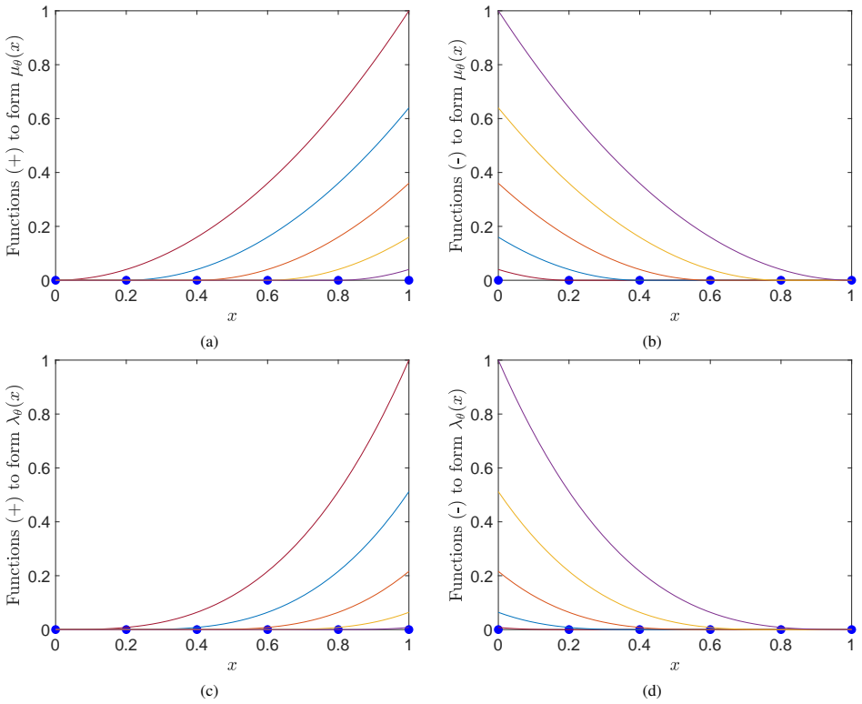
- For steady convection-diffusion, the numerical rates are approximately $p$ in the $L^2$ norm for $u$ and $p+1$ in the $H^1$ seminorm for $u'$ when the dual field $\mu$ has degree $p$ and $\lambda$ has degree $p+1$.
- Because the highest-order derivatives in the dual problem belong to heat or linear transport, the corresponding dual boundary-value problem is degenerate elliptic yet has a unique solution, covering the pure-transport limit.
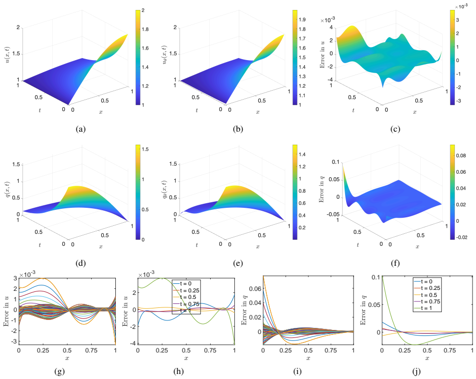
- Errors that concentrate near the terminal time $t=1$ are attributed to a corner conflict between dual Dirichlet data and can, per the paper, be removed by extending the time interval with a buffer zone or by time-slicing.
Reading between the lines
- Editorial inference: if the terminal boundary-layer errors are as localized as the examples suggest, the buffer-zone and time-slicing remedies make the space-time dual method practical for long-time simulation, but the paper does not demonstrate that combination with a convergence study.
- Editorial inference: the method's tolerance of linearly dependent RePU trial functions implies that overcomplete dictionaries can be used harmlessly as dual ansatz spaces, which could simplify constructing admissible neural-network trial spaces beyond standard basis constraints.
- Editorial inference: the same constraint-plus-convex-potential construction could turn parameter identification or inverse problems into convex dual optimization, since the primal equation enters only as a constraint; this direction is not explored here.
Editorial analysis
A structured set of objections, weighed in public.
Referee Report
Summary. The paper develops a duality-based variational formulation for PDEs that lack a primal variational structure, treating the PDE as a constraint and optimizing a user-chosen convex auxiliary potential. For the one-dimensional transient convection-diffusion equation, the authors derive a dual functional whose first variation is claimed to reproduce the primal weak form after the dual-to-primal map is substituted. They discretize the resulting symmetric variational problem with shallow RePU neural networks and B-splines in steady state, and with tensor-product B-splines in a space-time setting for transient problems. Numerical examples include Laplace's equation, steady-state and transient convection-diffusion, and transient heat conduction, together with a uniqueness proof for the dual variational system and numerical convergence studies for the steady-state problem.
Significance. If its claims hold, the paper offers a systematic way to obtain symmetric Galerkin formulations for non-variational PDEs without stabilization parameters, and it extends the dual approach to space-time discretizations using smooth approximants. The explicit stiffness-matrix derivations in Section 4, the uniqueness proof in Section 4.1, and the exact recovery of the Laplace solution in Section 5.1 are genuine strengths, as are the bracketing of the arbitrary terminal dual condition in the ODE example and the numerical convergence rates for the steady-state convection-diffusion problem. However, the transient results, which are the most novel contribution, currently carry an acknowledged terminal-time boundary-layer error whose proposed remedy is not implemented or tested; this weakens the paper's broad accuracy claim until the issue is resolved.
major comments (2)
- [Section 5.3 and 5.3.1] The main time-dependent demonstration reports relative maximum errors of 0.06 for u and 0.1 for q, with the errors explicitly concentrated near the terminal time t=1. The paper attributes this to the corner conflict caused by the arbitrarily chosen terminal condition λ(x,1)=0 and then proposes a buffer-zone extension of the time domain to [0,T+δ], discarding (T,T+δ], but this remedy is never implemented or tested. Moreover, no h- or p-refinement study is reported for the transient convection-diffusion problem, so it is not demonstrated that the contamination is localized and decreases with resolution. Because the abstract claims that the method 'delivers sound accuracy for ODEs and PDEs,' this transient accuracy claim is load-bearing and currently rests on an untested assumption. Please implement the buffer-zone or time-slicing strategy and report errors on the original interval [0,T], or provide a refinement study for the space-time discretization showing that the terminal-layer error is confined and reduced under refinement.
- [Section 3.2, Eq. (46)] The central theoretical step is the statement that the vanishing first variation of the dual functional S[λ,μ] is, up to Dirichlet conditions on λ, the weak form of the primal IBVP with the dual-to-primal map incorporated. The paper delegates this to 'familiar lines' and does not show the explicit integration-by-parts calculation. Since this equivalence is the foundation of the numerical discretization in Section 4 and also clarifies why λ may be assigned a terminal condition while u cannot, please include the full derivation, showing how the boundary data u1,u2 and the initial condition u0 arise as natural conditions from (53)-(54). This will also make precise the sense in which the top-edge dual boundary condition creates the terminal boundary layer discussed in Section 5.3.1.
minor comments (5)
- [Eq. (52a)] The tuple D in the transient heat equation should contain ∂μ/∂x, not ∂u/∂x; as written, it is inconsistent with the dual-to-primal map used in (52a).
- [Abstract and Section 5.2.2] The abstract says rates of convergence are 'established,' but the paper provides numerically observed slopes and heuristic interpolation estimates rather than a convergence theorem; please qualify the claim as numerical or provide a proof.
- [Section 5.2.1] The RePU 'neural network' approximants have fixed hidden-layer weights and biases, so only the output-layer coefficients are unknown and the approximation is linear in the unknowns; this should be stated explicitly at the first use to avoid overclaiming a machine-learning training procedure.
- [Section 4.1] The integral notation ∫_0^1∫_t^1 ... is confusing because t is used both as the time variable and as the lower limit of integration; replacing the inner integration variable with τ would improve readability.
- [Figure 13] For α=50 with p=q=1, the reported rates (1.2, 0.9) are not close to the predicted order one; a sentence explaining the effect of the boundary layer on the coarsest discretizations would help.
Circularity Check
No significant circularity: the dual variational method is a constructed reformulation, and the numerical validations are independent of the framework's own claims.
full rationale
The paper's central equivalence (abstract; Section 3.2, Eqs. (46)-(55)) is a genuine Lagrange-duality construction: the primal PDE system (36)-(37) is appended to a convex potential H via multipliers λ and µ; the stationarity conditions ∂L/∂u=0 and ∂L/∂q=0 yield the explicit dual-to-primal map (44b); substituting this map into the pre-dual functional produces a dual functional S[λ,µ] whose first variation, after integration by parts, is exactly the weak form of the primal PDE with the DtP change of variables incorporated. This is an algebraic identity, not an input-output circularity: the 'prediction' is the numerical solution of a well-posed boundary-value problem for (λ,µ), compared against independent exact solutions (e.g., Eqs. (61c), (68d), (72d)). The arbitrary dual Dirichlet data are explicitly shown not to determine the primal solution in the IVP example (Eqs. (31)-(35)), where the λ(T) dependence cancels identically. The uniqueness proof in Section 4.1 is self-contained and does not import a load-bearing theorem from the authors' prior work. The convergence rates reported in Section 5.2 are observed numerical rates compared with standard interpolation estimates; they are not fitted parameters renamed as predictions. Self-citations to [9]-[18] provide background and prior demonstrations, but the present derivation is carried out in the text, so the citations are not load-bearing. The paper itself flags a real limitation in Section 5.3.1: errors grow near the terminal time t=1 due to a corner mismatch in the dual boundary data, and the proposed buffer-zone remedy is described but not implemented in this work, with the authors citing prior papers [17,18] for that remedy. This is a robustness gap and a correctness concern, but it is not a circularity, because it does not make the reported numerical results equal to the inputs by construction. Overall, the derivation chain is self-contained and the validations are against independent benchmarks, so the circularity score is low.
Assumptions & free parameters
free parameters (3)
- Auxiliary potential H =
H(u,q) = (u^2 + q^2)/2
- Polynomial degrees (p,q) for dual fields =
e.g., p=2,q=3; p=3,q=4; p=9,q=10
- Base state and weighting beta for quadratic-system example =
beta=10, base state (1,1)
assumptions (4)
- domain assumption Dual variational principle from [9-11]: Euler-Lagrange equations of the dual functional recover the primal PDE with the dual-to-primal map.
- domain assumption The auxiliary potential H is strongly convex and dominates nonlinearities so the DtP map is well-defined.
- domain assumption Arbitrary Dirichlet data on the dual field lambda do not affect the exact primal solution.
- domain assumption Standard interpolation estimates apply to the Galerkin method, giving O(h^p) in L2 and O(h^{p+1}) in H1 rates.
Cite this review
Pith. "Pith review of Variational formulation based on duality to solve partial differential equations: Use of B-splines and machine learning approximants." pith.science (2026). https://pith.science/paper/ZNQCLJPZ
@misc{pith2026241201232,
  author       = {Pith},
  title        = {Pith review of: Variational formulation based on duality to solve partial differential equations: Use of B-splines and machine learning approximants},
  year         = {2026},
  howpublished = {\url{https://pith.science/paper/ZNQCLJPZ}},
  note         = {Machine review of arXiv:2412.01232}
}
abstract
Many partial differential equations (PDEs) such as Navier--Stokes equations in fluid mechanics, inelastic deformation in solids, and transient parabolic and hyperbolic equations do not have an exact, primal variational structure. Recently, a variational principle based on the dual (Lagrange multiplier) field was proposed. The essential idea in this approach is to treat the given PDEs as constraints, and to invoke an arbitrarily chosen auxiliary potential with strong convexity properties to be optimized. On requiring the vanishing of the gradient of the Lagrangian with respect to the primal variables, a mapping from the dual to the primal fields is obtained. This leads to requiring a convex dual functional to be minimized subject to Dirichlet boundary conditions on dual variables, with the guarantee that even PDEs that do not possess a variational structure in primal form can be solved via a variational principle. The vanishing of the first variation of the dual functional is, up to Dirichlet boundary conditions on dual fields, the weak form of the primal PDE problem with the dual-to-primal change of variables incorporated. We derive the dual weak form for the linear, one-dimensional, transient convection-diffusion equation. A Galerkin discretization is used, with the trial and test functions chosen as linear combination of either shallow neural networks with RePU activation functions or B-splines; the corresponding stiffness matrix is symmetric. For transient problems, a space-time Galerkin implementation is used with tensor-product B-splines as approximating functions. Numerical results are presented for the steady-state and transient convection-diffusion equation, and transient heat conduction. The proposed method delivers sound accuracy for ODEs and PDEs and rates of convergence are established in the $L^2$ norm and $H^1$ seminorm for the steady-state convection-diffusion problem.
Figures


Figures from the paper (16 more)


Reference graph
Works this paper leans on
-
[1]
N. Ghoussoub, A. Moameni, Anti-symmetric Hamiltonians (II): Variational resolutions for Navier–Stokes and other nonlinear evolutions, Annales de l’Institut Henri Poincar´e C 26 (1) (2009) 223–255
work page 2009
- [2]
- [3]
- [4]
-
[5]
H. Petryk, A quasi-extremal energy principle for non-potential problems in rate-independent plasticity, Journal of the Mechanics and Physics of Solids 136 (2020) 103691
work page 2020
-
[6]
C. Carstensen, K. Hackl, A. Mielke, Non–convex potentials and microstructures in finite–strain plasticity, Proceedings of the Royal Society of London. Series A: Mathematical, Physical and Engineering Sciences 458 (2018) (2002) 299–317
work page 2018
-
[7]
M. Gurtin, Variational principles for linear initial-value problems, Quarterly of Applied Mathematics 22 (3) (1964) 252–256
work page 1964
-
[8]
R. L. Seliger, G. B. Whitham, Variational principles in continuum mechanics, Proceedings of the Royal Society of London. Series A. Mathe- matical and Physical Sciences 305 (1480) (1968) 1–25
work page 1968
Show all 47 references
-
[9]
Acharya, Variational principle for nonlinear PDE systems via duality, Quarterly of Applied Mathematics 81 (2023) 127–140
A. Acharya, Variational principle for nonlinear PDE systems via duality, Quarterly of Applied Mathematics 81 (2023) 127–140
2023
-
[10]
Acharya, A dual variational principle for nonlinear dislocation dynamics, Journal of Elasticity 154 (1) (2023) 383–395
A. Acharya, A dual variational principle for nonlinear dislocation dynamics, Journal of Elasticity 154 (1) (2023) 383–395
2023
-
[11]
A. Acharya, A hidden convexity in continuum mechanics, with application to classical, continuous-time, rate-(in) dependent plasticity, Math- ematics and Mechanics of Solids 30 (3) (2025) 701–719, arXiv:2310.03201 (2024)
2025 arXiv
-
[12]
Singh, J
S. Singh, J. Ginster, A. Acharya, A hidden convexity of nonlinear elasticity, Journal of Elasticity 156 (2024) 975–1014
2024
-
[13]
Acharya, B
A. Acharya, B. Stro ffolini, A. Zarnescu, Variational dual solutions for incompressible fluids (2024). arXiv:2409.04911. 43
2024
-
[14]
Acharya, A
A. Acharya, A. N. Sengupta, Action principles for dissipative, non-holonomic Newtonian mechanics, Proceedings of the Royal Society of London. Series A, Mathematical and Physical Sciences 480 (2024) 20240113
2024
-
[15]
R. M. Errico, What is an adjoint model?, Bulletin of the American Meteorological Society 78 (11) (1997) 2577–2591
1997
-
[16]
Y . Cao, S. Li, L. Petzold, R. Serban, Adjoint sensitivity analysis for differential-algebraic equations: The adjoint DAE system and its numerical solution, SIAM Journal on Scientific Computing 24 (3) (2003) 1076–1089
2003
-
[17]
Kouskiya, A
U. Kouskiya, A. Acharya, Hidden convexity in the heat, linear transport, and Euler’s rigid body equations: A computational approach, Quarterly of Applied Mathematics 82 (2024) 673–703
2024
-
[18]
Kouskiya, A
U. Kouskiya, A. Acharya, Inviscid Burgers as a degenerate elliptic problem, published online, Quarterly of Applied Mathematics ( https: //arxiv.org/abs/2401.08814, 2024)
2024 arXiv
-
[19]
Brenier, Hidden convexity in some nonlinear PDEs from geomety and physics, Journal of Convex Analysis 17 (3&4) (2010) 945–959
Y . Brenier, Hidden convexity in some nonlinear PDEs from geomety and physics, Journal of Convex Analysis 17 (3&4) (2010) 945–959
2010
-
[20]
Y . Brenier, The initial value problem for the Euler equations of incompressible fluids viewed as a concave maximization problem, Communi- cations in Mathematical Physics 364 (2018) 579–605
2018
-
[21]
A. N. Brooks, T. J. R. Hughes, Streamline upwind /Petrov–Galerkin formulations for convection dominated flows with particular emphasis on the incompressible Navier–Stokes equations, Computer Methods in Applied Mechanics and Engineering 32 (1-3) (1982) 199–259
1982
-
[22]
T. J. R. Hughes, L. P. Franca, P. Leopoldo, G. M. Hulbert, A new finite element formulation for computational fluid dynamics: VIII. The Galerkin/least-squares method for advective-di ffusive equations, Computer Methods in Applied Mechanics and Engineering 73 (2) (1989) 173–189
1989
-
[23]
T. E. Tezduyar, Stabilized finite element formulations for incompressible flow computations, Advances in Applied Mechanics 28 (1991) 1–44
1991
-
[24]
T. J. R. Hughes, Multiscale phenomena: Green’s functions, the Dirichlet-to-Neumann formulation, subgrid scale models, bubbles and the origins of stabilized methods, Computer Methods in Applied Mechanics and Engineering 127 (1-4) (1995) 387–401
1995
-
[25]
P. B. Bochev, M. D. Gunzburger, Least-Squares Finite Element Methods, V ol. 166, Springer Science & Business Media, 2009
2009
-
[26]
Raissi, P
M. Raissi, P. Perdikaris, G. E. Karniadakis, Physics-informed neural networks: A deep learning framework for forward and inverse problems involving nonlinear partial differential equations, Journal of Computational Physics 378 (2019) 686–707
2019
-
[27]
G. E. Karniadakis, I. G. Kevrekidis, L. Lu, P. Perdikaris, S. Wang, L. Yang, Physics-informed scientific machine learning, Nature Review Physics 3 (6) (2021) 422–440
2021
-
[28]
Cuomo, V
S. Cuomo, V . S. Di Cola, F. Giampaolo, G. Rozza, M. Raissi, F. Piccialli, Scientific machine learning through physics-informed neural networks: Where we are and what’s next, Journal of Scientific Computing 92 (3) (2022) 88
2022
-
[29]
Z. Liu, Y . Wang, S. Vaidya, F. Ruehle, J. Halverson, M. Solja ˇci´c, T. Y . Hou, M. Tegmark, KAN: Kolmogorov–Arnold networks (2024). arXiv:2404.19756
2024 arXiv
-
[30]
B. C. Koenig, S. Kim, S. Deng, KAN-ODEs: Kolmogorov–Arnold network ordinary di fferential equations for learning dynamical systems and hidden physics (2024). arXiv:2407.04192
2024 arXiv
-
[31]
L. F. Guilhoto, P. Perdikaris, Deep learning alternatives of the Kolmogorov superposition theorem (2024). arXiv:2410.01990
2024 arXiv
-
[32]
W. E, B. Yu, The deep Ritz method: A deep learning-based numerical algorithm for solving variational problems, Communications in Mathematics and Statistics 6 (1) (2018) 1–12
2018
-
[33]
Sukumar, A
N. Sukumar, A. Srivastava, Exact imposition of boundary conditions with distance functions in physics-informed deep neural networks, Computer Methods in Applied Mechanics and Engineering 389 (2022) 114333
2022
-
[34]
J. He, J. Xu, Expressivity and approximation properties of deep neural networks with ReLU k activation (2024). arXiv:2312.16483
2024 arXiv
-
[35]
J. He, J. Xu, Deep neural networks and finite elements of any order on arbitrary dimensions (2024). arXiv:2312.14276
2024 arXiv
-
[36]
de Boor, A Practical Guide to Splines, Applied Mathematical Sciences, Springer, New York, 2001
C. de Boor, A Practical Guide to Splines, Applied Mathematical Sciences, Springer, New York, 2001
2001
-
[37]
M. S. Floater, Generalized barycentric coordinates and applications, Acta Numerica 24 (2015) 161–214
2015
-
[38]
C. E. Shannon, A mathematical theory of communication, The Bell System Technical Journal 27 (1948) 379–423
1948
-
[39]
E. T. Jaynes, Information theory and statistical mechanics, Physical Review 106 (4) (1957) 620–630
1957
-
[40]
Sukumar, Construction of polygonal interpolants: a maximum entropy approach, International Journal for Numerical Methods in Engi- neering 61 (12) (2004) 2159–2181
N. Sukumar, Construction of polygonal interpolants: a maximum entropy approach, International Journal for Numerical Methods in Engi- neering 61 (12) (2004) 2159–2181
2004
-
[41]
Belytschko, Y
T. Belytschko, Y . Krongauz, D. Organ, M. Fleming, P. Krysl, Meshless methods: An overview and recent developments, Computer Methods in Applied Mechanics and Engineering 139 (1996) 3–47
1996
-
[42]
T. M. Black, Mesh-free Applications to Fracture Mechanics and An Analysis of the Corrected Derivative Method, Ph.D. thesis, Theoretical and Applied Mechanics, Northwestern University, Evanston, IL, U.S.A. (December 1999)
1999
-
[43]
Punzo, A
F. Punzo, A. Tesei, Uniqueness of solutions to degenerate elliptic problems with unbounded coe fficients, Annales de l’Institut Henri Poincar´e C 26 (5) (2009) 2001–2024
2009
-
[44]
T. J. R. Hughes, The Finite Element Method: Linear Static and Dynamic Finite Element Analysis, Prentice-Hall, Englewood Cli ffs, N.J., 1987
1987
-
[45]
M. B. Glinowiecka-Cox, Analytic Solution of 1D Diffusion-Convection Equation with Varying Boundary Conditions, B.S. Thesis, Department of Mathematics, Portland State University, Portland, OR 97207, USA (2022)
2022
-
[46]
Acharya, J
A. Acharya, J. Ginster, A. N. Sengupta, Variational dual solutions of Chern-Simons theory (2024). arXiv:2411.17635
2024 arXiv
-
[47]
A. M. Bradley, A tutorial on the adjoint method (2024). URL https://cs.stanford.edu/~ambrad/adjoint_tutorial.pdf 44
2024
Reviewed August 12, 2026 · model on record in the stance chip above.
Discussion (0). Continue with ORCID to comment.