REVIEW 3 major objections 3 minor 17 references
Modular addition without black-boxes: Compressing explanations of MLPs that compute numerical integration
T0 review · 3 major / 3 minor · reviewed 2026-08-11 · deepseek-v4-flash
Pith's one-line read The ReLU MLP in a modular-addition transformer is best understood as a quadrature scheme, and this interpretation yields non-vacuous error bounds in time linear in the parameter count.
desk verdict A genuinely new interpretation of the ReLU MLP in pizza-algorithm transformers, with an honest but incomplete non-vacuous bound; worth refereeing. read the letter →
The pith
A machine-rendered reading of the paper's core claim, the machinery that carries it, and where it could break.
The reading
What carries the argument
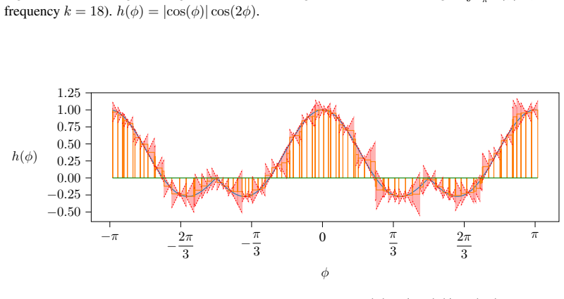
The central object is the quadrature scheme: the finite neuron sum is read as a Riemann-style integral over the phase variable $\phi$. The key identity is $\int_{-\pi}^{\pi} \mathrm{ReLU}[\sigma_k \cos(k(a+b)/2 + \phi)] \cos(kc + 2\phi)\,d\phi = \frac{2}{3}\cos(k(a+b-c))$. The mechanism that makes the reduction work is the amplitude-phase Fourier representation of the model's weight matrices, which reveals that each neuron has a single dominant frequency $k$, that its output phase is approximately double its input phase ($\psi_i \approx 2\phi_i$), and that the phases are roughly uniformly distributed; those facts justify grouping neurons into clusters $I_k$ and replacing each cluster's sum by an integral. To bound the error in linear time, the paper splits ReLU into its identity part $x/2$, whose integral vanishes, and its absolute-value part $|x|/2$, whose Lipschitz constant bounds the rectangle error via $\sup |h'| \le 2$.
What would settle it
Train the same constant-attention one-layer transformer on modular addition with a different modulus or width and inspect the phase plot for each key-frequency cluster: if any cluster that still solves the task has the $\psi_i \approx 2\phi_i$ regression with $R^2$ below 0.9, the quadrature interpretation is not the mechanism. Equivalently, compute the paper's relative error bound on a trained model and look for any input triple $(a,b,c)$ where it exceeds 1.
Extended reading notes
Core claim
On the paper's own terms, the central discovery is that the trained MLP layer computes the pizza algorithm's frequency-doubling step by numerical quadrature, not by an opaque feature interaction. For each key frequency $k$, neurons cluster into a group $I_k$; after sorting their input phases $\phi_i$, the normalized MLP output $\sum_{i\in I_k} w_i\, \mathrm{ReLU}[\sigma_k \cos(k(a+b)/2 + \phi_i)] \cos(kc + 2\phi_i)$ is a rectangle-rule approximation to the integral in Eq. (5), which equals $\frac{2}{3}\cos(k(a+b-c))$. The paper establishes the structure by amplitude-phase Fourier analysis: most neurons are dominated by a single key frequency, and the output phase $\psi_i$ is almost exactly twice the input phase $\phi_i$, with $R^2 > 0.99$. It then validates the interpretation by computing relative error bounds between 0.48 and 0.70 for the mainline model, all strictly below 1, in time $O(d_{\text{mlp}} + p)$, and shows the phenomenon recurs across 100 of 151 randomly seeded models.
Load-bearing premise
The argument rests on an empirical regularity rather than a proven theorem: in a trained model, each neuron is dominated by a single key frequency and its output phase is almost exactly twice its input phase; if that pattern breaks, the clustering into $I_k$ and the reduction to Eq. (5) collapse.
Editorial extensions
If this is right
- Verifying the MLP's behavior no longer requires enumerating all $p^2$ input pairs; the paper's bound runs in $O(d_{\text{mlp}} + p)$ time, which is linear in the parameter count.
- Splitting ReLU into identity plus absolute-value parts shows the nonlinear part alone implements the pizza logits, while the identity part is exactly compressible through a matrix $A$ with $\mathrm{logit} = A[:,a] + A[:,b]$.
- Secondary frequencies equal to twice each key frequency produce a $-\frac{\pi}{2}\cos(k(a-b))\cos(k(a+b-c))$ correction that compensates for the pizza algorithm's weakness when $|\cos(k(a-b)/2)| \approx 0$, explaining why overall logits regress better against the clock form.
- Across 100 'good' models from 151 random seeds, 82% of (model, frequency) pairs have empirical integration errors below 0.1, and the median normalized bound is 0.40 versus a naive baseline of 0.85.
- The same quadrature-error machinery applies to both signs $\sigma_k = \pm 1$ because the integral identity holds for both, so the bound covers all inputs without case-splitting.
Reading between the lines
- Because the paper only trains with modulus $p=59$, a direct testable extension is to check whether the single-frequency and phase-doubling regularity persists at larger moduli; if it does, the same $O(d_{\text{mlp}}+p)$ bound should hold there.
- The rectangle-error argument relies only on a bounded derivative and sorted phases, so a similar quadrature compression may apply to other pointwise nonlinearities with bounded Lipschitz constants, not just ReLU.
- The paper's split of ReLU into an exactly compressible linear part and a quadrature-compressible nonlinear residual suggests a general recipe for compressing nonlinear layers: isolate the linear component, then integrate the nonlinear residual.
- If larger transformers show 'clock-like' logit regressions, the secondary-frequency compensation mechanism implies that the underlying computation may still be pizza-like; a purely logit-level regression cannot distinguish the two algorithms.
Editorial analysis
A structured set of objections, weighed in public.
Referee Report
Summary. This paper studies one-layer constant-attention ReLU transformers trained on modular addition (the 'pizza' models of Zhong et al.). The authors propose that the MLP layer implements frequency doubling by numerical quadrature: after sorting neurons by their input phase φ_i, the sum over neurons is interpreted as a Riemann sum for the integral ∫ ReLU[σ_k cos(k(a+b)/2 + φ)] cos(kc + 2φ) dφ = (2/3) cos(k(a+b-c)). They support this with empirical phase-amplitude observations (single-frequency dominance, ψ_i ≈ 2φ_i), an analytic derivation of the integral identity, and computed quadrature error bounds (Tables 1–3) that are non-vacuous (relative error bounds 0.48–0.70) and computable in time linear in the number of neurons. The paper also explains how secondary frequencies at 2k improve robustness when |cos(k(a-b)/2)| is small.
Significance. If the full claimed result were established, this would be an important step in mechanistic interpretability: a rigorous, non-vacuous, linear-time-certifiable compression of a nonlinear MLP feature map, going beyond prior black-box descriptions. The analytic integral identity in Appendix E is clean and parameter-free, and the empirical quadrature errors (0.03–0.05) are convincingly small. The systematic validation across 151 training runs and the released code are strengths. However, the significance is currently undercut by the gap between the bound that is proved and the bound that is advertised; the non-vacuous certificate is for an idealized primary-frequency model, not for the full trained MLP.
major comments (3)
- [§5, Appendix L.2] The non-vacuous bound advertised in the abstract and Section 5 is not a bound on the full ReLU MLP. Equation (13) and Table 1 bound the quadrature error of the idealized sum in Eq. (4), in which each neuron has been replaced by its primary Fourier component and the output phase is set to exactly 2φ_i. The projection error between the actual MLP and this idealized sum is not bounded: the identity component of ReLU, the residual-stream terms (OVE on x and y, the MLP bias, the embed of y), the secondary frequencies, and the non-primary components of W_L are all excluded. Appendix L.2 states this explicitly ('To bound the error of our interpretation of the MLP precisely, we'd need to include a bound on the primary frequency contribution of the identity component...'). Tables 2 and 3 report errors and bounds for the h-functions, not for the model logits. The abstract's claim of 'a non-vacuous bound on the behaviour of the ReLU MLP' is therefore not supported; at present the paper provides a non-vacuous bound on a component of an idealized version of the MLP.
- [§5.2, Table 3, Appendix H] The empirical 'Normalised ... error' rows are brute-force evaluations of the h-function quadrature error, not worst-case bounds on the model's logits, and the 'Total numerical ... bound' rows are bounds for the same h-functions. Reporting these as evidence that 'the model is indeed performing numerical integration' conflates an empirical fit with a formal guarantee. Moreover, the R² statistics in Figures 3 and 4 are aggregate goodness-of-fit measures; they do not certify the worst-case accuracy of the phase-doubling and single-frequency assumptions on which the bound's validity depends. The paper should either present a bound that covers the full logit expression or explicitly narrow the claim to the idealized primary-frequency model throughout the abstract and introduction.
- [§4.3, Eq. (4), Appendix C] The reduction to Eq. (4) assumes that every neuron can be assigned to a single key frequency cluster I_k and that the output phase satisfies ψ_i = 2φ_i. These are empirical observations, not theorems, and the coverage is incomplete: Appendix C reports that only 100 of 151 models are 'good' (frequency matching for all neurons), and for many of these the phase R² or the uniformity of angle widths falls below the thresholds. The error bound in §5 inherits the projection error from any neuron that does not satisfy these assumptions, and the paper does not quantify that error for the excluded models. The main text should state these coverage limitations and their impact on the validity of the bound.
minor comments (3)
- [§4.3, Eq. (4)] The phrase 'can we well-thought of as approximating the integral' should read 'can be thought of as approximating the integral'.
- [Figure 2 caption] The caption says 'The MLP approximately computes the integral', but the plotted h(φ) is not the full MLP output; consider rephrasing to 'the primary-frequency absolute-value component is approximated by the integral'.
- [§5.1, Eq. (13)] The displayed formula mixes the case distinction with the absolute value; adding a short derivation of the interval integral would improve readability.
Circularity Check
No significant circularity: the trigonometric integral identity and quadrature error bound are derived independently of the fitted model, though the paper's compression criterion is self-cited and the headline MLP bound currently covers only the idealized primary-frequency absolute-value part.
full rationale
The paper's core derivation is self-contained rather than circular. The integral identity in Eq. (5), ∫ ReLU[σ_k cos(k(a+b)/2 + φ)] cos(kc + 2φ) dφ = (2/3) cos(k(a+b−c)), is derived in Appendix E from standard trigonometric identities with no dependence on trained weights. The empirical regularities that drive the interpretation—single-frequency dominance, ψ_i ≈ 2φ_i, and roughly uniform phase spacing—are discovered from Fourier analysis of the trained models (Section 4.2, Figures 3–4) and are not imposed to force Eq. (6). The Section 5 error bound is a genuine mathematical upper bound on the quadrature error of the idealized sum in Eq. (4); it is computed from the model's extracted phases and weights plus the analytic bound sup|h'| ≤ 2, and it holds uniformly over a, b, c in O(d_mlp + p) time. This is not a fitted parameter renamed as a prediction, because the weights and phases are model parameters rather than free parameters optimized to match the integral. The main caveat is scope, not circularity: as Appendix L.2 explicitly states, 'To bound the error of our interpretation of the MLP precisely, we'd need to include a bound on the primary frequency contribution of the identity component... and include bounds on the residual components,' so the advertised bound on 'the behaviour of the ReLU MLP' is presently a bound on the idealized primary-frequency absolute-value part, not the full trained MLP. That is an admitted omitted proof/limitation and a correctness risk, but it does not make the derivation circular. The only self-referential element is the framing target from Gross et al. (2024), whose authors overlap with four of the five authors of this paper; the 'non-vacuous bound in linear time' criterion is imported from that work, but it is a formalization choice rather than a load-bearing theorem, and the trigonometric and quadrature analysis stands independently of it. Overall, no step of the derivation reduces by construction to its own inputs; the observed model structure is an input to the interpretation, and the integral identity and bound are evaluated against that structure rather than derived from it.
Assumptions & free parameters
free parameters (7)
- Key frequency set K (mainline: 12, 18, 21, 22) =
12, 18, 21, 22 (multiplied by 2π/p)
- Per-neuron primary frequency assignment I_k =
varies per model
- Neuron input phases φ_i =
not tabulated
- Neuron output phases ψ_i =
ψ_i ≈ 2φ_i, R2 > 0.99
- Quadrature weights w'_i (rectangle widths) =
not tabulated
- Per-frequency normalization or scale Z_k =
empirical, not tabulated
- Secondary frequency coefficients β_i and phase offsets =
φ_2 ≈ 2φ_1 + π, R2 > 0.99
assumptions (5)
- domain assumption Trained one-layer constant-attention transformers trained on modular addition implement the pizza frequency-doubling algorithm as characterized by Zhong et al. (2023).
- ad hoc to paper The infinite-width lens conditions hold: there exists a neuron-indexed integration variable ξ such that weights are approximately linear in node spacing and the integrand is sufficiently continuous.
- domain assumption For each neuron, the largest Fourier component of the pre-activation and of the corresponding WL row share the same frequency, and the output phase is twice the input phase.
- domain assumption Residual stream and identity-component contributions can be bounded separately and are small enough not to invalidate the compressed explanation.
- standard math Standard trigonometric identities and the Lipschitz bound on the derivative of h are used in the quadrature error analysis.
Cite this review
Pith. "Pith review of Modular addition without black-boxes: Compressing explanations of MLPs that compute numerical integration." pith.science (2026). https://pith.science/paper/FS63F4S3
@misc{pith2026241203773,
  author       = {Pith},
  title        = {Pith review of: Modular addition without black-boxes: Compressing explanations of MLPs that compute numerical integration},
  year         = {2026},
  howpublished = {\url{https://pith.science/paper/FS63F4S3}},
  note         = {Machine review of arXiv:2412.03773}
}
read the original abstract
The goal of mechanistic interpretability is discovering simpler, low-rank algorithms implemented by models. While we can compress activations into features, compressing nonlinear feature-maps -- like MLP layers -- is an open problem. In this work, we present the first case study in rigorously compressing nonlinear feature-maps, which are the leading asymptotic bottleneck to compressing small transformer models. We work in the classic setting of the modular addition models, and target a non-vacuous bound on the behaviour of the ReLU MLP in time linear in the parameter-count of the circuit. To study the ReLU MLP analytically, we use the infinite-width lens, which turns post-activation matrix multiplications into approximate integrals. We discover a novel interpretation of} the MLP layer in one-layer transformers implementing the ``pizza'' algorithm: the MLP can be understood as evaluating a quadrature scheme, where each neuron computes the area of a rectangle under the curve of a trigonometric integral identity. Our code is available at https://tinyurl.com/mod-add-integration.
Figures


Figures from the paper (36 more)




Reference graph
Works this paper leans on
-
[1]
Interpreting neural networks through the polytope lens, 2022
Sid Black, Lee Sharkey, Leo Grinsztajn, Eric Winsor, Dan Braun, Jacob Merizian, Kip Parker, Carlos Ramón Guevara, Beren Millidge, Gabriel Alfour, and Connor Leahy. Interpreting neural networks through the polytope lens, 2022
work page 2022
-
[2]
Towards monosemanticity: Decomposing language models with dictionary learning
Trenton Bricken, Adly Templeton, Joshua Batson, Brian Chen, Adam Jermyn, Tom Conerly, Nick Turner, Cem Anil, Carson Denison, Amanda Askell, Robert Lasenby, Yifan Wu, Shauna Kravec, Nicholas Schiefer, Tim Maxwell, Nicholas Joseph, Zac Hatfield-Dodds, Alex Tamkin, Karina Nguyen, Brayden McLean, Josiah E Burke, Tristan Hume, Shan Carter, Tom Henighan, and Ch...
2023
-
[3]
Sparse autoencoders find highly interpretable features in language models, 2023
Hoagy Cunningham, Aidan Ewart, Logan Riggs, Robert Huben, and Lee Sharkey. Sparse autoencoders find highly interpretable features in language models, 2023. URL https://arxiv.org/abs/2309.08600
arXiv 2023
-
[4]
A mathematical framework for transformer circuits
Nelson Elhage, Neel Nanda, Catherine Olsson, Tom Henighan, Nicholas Joseph, Ben Mann, Amanda Askell, Yuntao Bai, Anna Chen, Tom Conerly, Nova DasSarma, Dawn Drain, Deep Ganguli, Zac Hatfield-Dodds, Danny Hernandez, Andy Jones, Jackson Kernion, Liane Lovitt, Kamal Ndousse, Dario Amodei, Tom Brown, Jack Clark, Jared Kaplan, Sam McCandlish, and Chris Olah. A...
2021
-
[5]
Toy models of superposition
Nelson Elhage, Tristan Hume, Catherine Olsson, Nicholas Schiefer, Tom Henighan, Shauna Kravec, Zac Hatfield-Dodds, Robert Lasenby, Dawn Drain, Carol Chen, Roger Grosse, Sam McCandlish, Jared Kaplan, Dario Amodei, Martin Wattenberg, and Christopher Olah. Toy models of superposition. Transformer Circuits Thread, 2022. URL https://transformer-circuits.pub/20...
2022
-
[6]
Michaud, Wes Gurnee, and Max Tegmark
Joshua Engels, Isaac Liao, Eric J. Michaud, Wes Gurnee, and Max Tegmark. Not all language model features are linear, 2024. URL https://arxiv.org/abs/2405.14860
arXiv 2024
-
[7]
Grokking modular arithmetic, 2023
Andrey Gromov. Grokking modular arithmetic, 2023. URL https://arxiv.org/abs/2301.02679
arXiv 2023
-
[8]
Compact proofs of model performance via mechanistic intepretability, June 2024
Jason Gross, Rajashree Agrawal, Thomas Kwa, Euan Ong, Chun Hei Yip, Alex Gibson, Soufiane Noubir, and Lawrence Chan. Compact proofs of model performance via mechanistic intepretability, June 2024. URL https://arxiv.org/abs/2406.11779
arXiv 2024
Show all 17 references
-
[9]
Michaud, Yonatan Belinkov, David Bau, and Aaron Mueller
Samuel Marks, Can Rager, Eric J. Michaud, Yonatan Belinkov, David Bau, and Aaron Mueller. Sparse feature circuits: Discovering and editing interpretable causal graphs in language models, 2024. URL https://arxiv.org/abs/2403.19647
2024 arXiv
-
[10]
Transformerlens
Neel Nanda and Joseph Bloom. Transformerlens. https://github.com/TransformerLensOrg/TransformerLens, 2022
2022
-
[11]
Progress measures for grokking via mechanistic interpretability
Neel Nanda, Lawrence Chan, Tom Lieberum, Jess Smith, and Jacob Steinhardt. Progress measures for grokking via mechanistic interpretability. arXiv preprint, 2023. doi:10.48550/arXiv.2301.05217. URL https://arxiv.org/abs/2301.05217
-
[12]
Zoom in: An introduction to circuits
Chris Olah, Nick Cammarata, Ludwig Schubert, Gabriel Goh, Michael Petrov, and Shan Carter. Zoom in: An introduction to circuits. Distill, 2020. doi:10.23915/distill.00024.001. URL https://distill.pub/2020/circuits/zoom-in
2020 doi
-
[13]
The clock and the pizza: Two stories in mechanistic explanation of neural networks, 2023
Ziqian Zhong, Ziming Liu, Max Tegmark, and Jacob Andreas. The clock and the pizza: Two stories in mechanistic explanation of neural networks, 2023. URL https://arxiv.org/abs/2306.17844
2023 arXiv
-
[14]
write newline
" write newline "" before.all 'output.state := FUNCTION n.dashify 't := "" t empty not t #1 #1 substring "-" = t #1 #2 substring "--" = not "--" * t #2 global.max substring 't := t #1 #1 substring "-" = "-" * t #2 global.max substring 't := while if t #1 #1 substring * t #2 gl...
-
[15]
@esa (Ref
\@ifxundefined[1] #1\@undefined \@firstoftwo \@secondoftwo \@ifnum[1] #1 \@firstoftwo \@secondoftwo \@ifx[1] #1 \@firstoftwo \@secondoftwo [2] @ #1 \@temptokena #2 #1 @ \@temptokena \@ifclassloaded agu2001 natbib The agu2001 class already includes natbib coding, so you should ...
-
[16]
\@lbibitem[] @bibitem@first@sw\@secondoftwo \@lbibitem[#1]#2 \@extra@b@citeb \@ifundefined br@#2\@extra@b@citeb \@namedef br@#2 \@nameuse br@#2\@extra@b@citeb \@ifundefined b@#2\@extra@b@citeb @num @parse #2 @tmp #1 NAT@b@open@#2 NAT@b@shut@#2 \@ifnum @merge>\@ne @bibitem@firs...
-
[17]
UjH敺 Um KJEd wؗɭ,ZZLPO <pJ ͐t wB` ?'(0 ZQoO2_ s Z / 4XV' 1n _ 0EP9> mߖĪQ!YϿ M - 5|P >8 _ Ə Wڷ I+A?M ^ P-- ExEqt=?l 5 7 u v / o I3< I V<pt UJ&gC4 j [r Z|댍> ,ve lV ` ă e
@open @close @open @close and [1] URL: #1 \@ifundefined chapter * \@mkboth \@ifxundefined @sectionbib * \@mkboth * \@mkboth\@gobbletwo \@ifclassloaded amsart * \@ifclassloaded amsbook * \@ifxundefined @heading @heading NAT@ctr thebibliography [1] @ \@biblabel @NAT@ctr \@bibset...
Reviewed August 11, 2026 · model on record in the stance chip above.
Discussion (0). Continue with ORCID to comment.