REVIEW 2 major objections 3 minor 46 references
Causal discovery with endogenous context variables
T0 review · 2 major / 3 minor · reviewed 2026-08-11 · deepseek-v4-flash
Pith's one-line read A modified PC algorithm provably recovers context-specific causal skeletons when the context indicator is endogenous.
desk verdict Solid theoretical contribution: a sound adaptive PC variant for endogenous context variables, but the physical-graph interpretation rests on an unverifiable identifiability assumption. read the letter →
The pith
A machine-rendered reading of the paper's core claim, the machinery that carries it, and where it could break.
The reading
What carries the argument
The central object is the context-specific graph triple ($G^{\mathrm{descr}}_{R=r}$, $G^{\mathrm{phys}}_{R=r}$, $G^{\mathrm{CF}}_{R=r}$) together with the adaptive test-selection rule. The rule determines, for every candidate separating set $S$, whether the independence is tested on the pooled data (if $R\notin S$) or per context (if $R\in S$). The load-bearing property is that, under weak context-sufficiency, physical mechanism changes are confined to children of $R$, while selection-bias-induced spurious links are confined to ancestors of $R$; with strong context-acyclicity these two sets do not overlap, so the rule never needs to test both ways on the same edge. The soundness proof uses the counterfactual graph to transfer d-separation in the context-specific DAG to a statement about the observed conditional distribution via counterfactual consistency.
What would settle it
Generate a system like the right-hand example of Sec. 3.2, where $P(T>T_0|R=0)<\epsilon$ makes $T\to Y$ disappear only because support is restricted, and run Algorithm 1 with oracle independence tests together with a direct check of whether $T$ remains a parent of $Y$ in the intervened mechanism $M_{\mathrm{do}(R=0)}$. If the algorithm removes $T\to Y$ while the physical graph keeps it, single-graph-sufficiency is violated and the physical interpretation is not valid.
Extended reading notes
Core claim
At the center of the paper is a distinction between three graphs associated with an SCM and a context value $r$: the descriptive graph (mechanisms in the intervened model, evaluated on the observed conditional support), the physical graph (mechanisms in the intervened model, evaluated on the full pooled support), and the counterfactual graph (what would be observed had $R$ been set to $r$ under the same noises). The paper's central claim is that a single adaptive decision rule lets a constraint-based algorithm recover the skeleton of the first two when they coincide. The rule is simple: for a candidate independence $X \perp\!\!\perp Y \mid S$, use the pooled test unless $R \in S$; when $R$ is in the conditioning set, test $X \perp\!\!\perp Y \mid S\setminus\{R\}, R=r$ inside each context. Theorem 1 states that in the oracle case, under causal sufficiency, single-graph-sufficiency, $R$-faithfulness, and strong context-acyclicity with minimal union cycles of length at most 2, Algorithm 1 recovers the skeleton of $G^{\mathrm{descr}}_{R=r}=G^{\mathrm{phys}}_{R=r}$. The paper also shows that without single-graph-sufficiency the output remains descriptively correct under weaker conditions, but should not be read as a physical mechanism change.
Load-bearing premise
The load-bearing premise is single-graph-sufficiency: within each context the descriptive, physical, and counterfactual graphs must coincide, so that an observed context-specific independence reflects a real mechanism change rather than merely a restricted region of the data.
Editorial extensions
If this is right
- A user who observes $R$ and satisfies the stated assumptions can replace an expensive masked search or an intersection-graph baseline with a single PC-style run that only occasionally goes per-context.
- The adaptive rule can be attached to other constraint-based algorithms, giving a general recipe for adding context-specific information to skeleton discovery under endogenous contexts.
- When single-graph-sufficiency fails, the algorithm still returns a graph between the descriptive and physical extremes; the correct interpretation is descriptive, not physical.
- The number of context-specific tests concentrates near $R$ and scales roughly linearly in the number of context variables, so the method remains feasible when many regimes are present.
Reading between the lines
- Editorial inference: a direct analogue of the decision rule should apply in time-series and FCI-style settings, where the context indicator's role as collider or ancestor determines whether per-context tests are safe; the paper notes the extension but does not develop it.
- Editorial inference: the support problem implies that a context-specific independence discovered by any conditional-independence test should be checked against the observational support of the conditioning variables, otherwise a descriptive edge removal may be mistaken for a physical mechanism change.
- Editorial inference: in parametric settings such as linear-Gaussian models per context, one could test single-graph-sufficiency directly by checking whether a link that vanishes per context corresponds to a zero coefficient in the intervened mechanism rather than to a restricted support.
Signed reviews
Editorial analysis
A structured set of objections, weighed in public.
Referee Report
Summary. The paper studies constraint-based causal discovery of context-specific causal graphs when the context variable R is endogenous. It introduces three graph notions (descriptive, physical, and counterfactual), identifies two failure modes (selection bias and the support problem), and proposes a hierarchy of context-sufficiency assumptions. The main result (Theorem 1) states that, under causal sufficiency, single-graph-sufficiency, R-faithfulness, and strong context-acyclicity with union cycles of length at most 2, an adaptive modification of PC (Algorithm 1) recovers the skeleton of G^descr_{R=r}=G^phys_{R=r}. The paper also presents a simulation study comparing the proposed method with masking, pooling, an intersection baseline, FCI-JCI0, and CD-NOD.
Significance. If the result holds, the paper makes a useful contribution by formalizing why naive masking or pooling can fail for endogenous contexts and by identifying sufficient conditions under which a simple adaptive testing rule is sound. The distinction between descriptive and physical context-specific graphs, and the explicit treatment of the support problem, are valuable and clearly presented. The proof of Theorem 1 is detailed, the assumptions are stated explicitly, and the code is provided. The main caveat, which the authors acknowledge, is that the physical interpretation depends on single-graph-sufficiency, an assumption that is not identifiable from the observable distribution.
major comments (2)
- [§4.2, Theorem 1 and §C, Definition C.2] The equality G^descr_{R=r}=G^phys_{R=r} in Theorem 1 is an input assumption, not a discovered property. Definition C.2 (single-graph-sufficiency) is not identifiable from P(V,R): as Example 3.2 can be modified to show, two SCMs can have identical P(V,R) but differ in whether a missing T->Y edge is due to an explicit mechanism change or to restricted support. The manuscript says this assumption is 'potentially harder to verify directly,' but it should state more strongly that no oracle independence test can distinguish the two cases. Please add an explicit non-identifiability statement (e.g., a proposition exhibiting two SCMs with the same P(V,R) and different G^phys) and temper the abstract/title wording so that the algorithm is described as recovering descriptive context-specific graphs, with physical interpretation only under an untestable assumption.
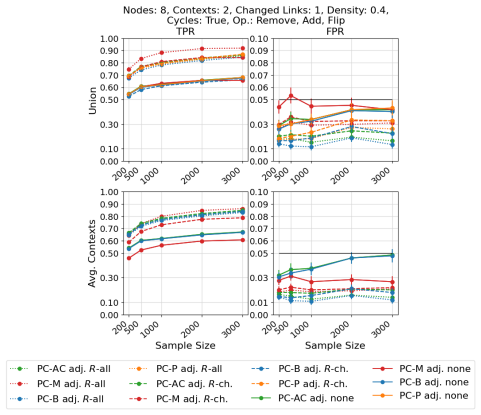
- [§5.1 and §E.1] The simulation study only generates SCMs that satisfy single-graph-sufficiency by construction: every edited variable is made a child of R, and operations add/remove/flip edges as explicit nonzero coefficients in the structural equations. The study therefore never includes support-problem instances of the kind illustrated in Example 3.2(ii), where G^descr_{R=r} differs from G^phys_{R=r} while P(V,R) is compatible. As a result, the finite-sample experiments do not probe the main limitation of the physical interpretation identified in §3.2. The authors should either add a synthetic support-problem scenario that violates single-graph-sufficiency (e.g., an edge removal due to restricted support rather than an explicit mechanism change) or at least explicitly state why such scenarios are excluded and how the method is expected to behave when they occur.
minor comments (3)
- [§4.1, Algorithm 1] In line 8, the notation 'S \ R, R= r' is ambiguous; it should read 'S \ {R}, R = r' to make clear that R is removed from the conditioning set and then set to the context value.
- [§5.2, Figure 3] The text refers to 'the left plot' and 'the right plot' of Figure 3, but the figure has two panels; 'left panel' and 'right panel' would be clearer.
- [§E.1] The data-generation description says that after each edit an edge from R to the affected child is added; the authors should explicitly note that this makes the generated models satisfy weak context-sufficiency, and in fact single-graph-sufficiency, by construction, since this is important context for interpreting the simulation results.
Circularity Check
No significant circularity: Theorem 1 is a conditional soundness result; the physical interpretation is imported by an explicit, honest assumption, not derived from the algorithm's own output.
full rationale
I find no circular step that reduces a prediction to an input. The central result (Theorem 1) is a conditional oracle-soundness theorem: under causal sufficiency, single-graph-sufficiency, R-faithfulness, and strong context-acyclicity with minimal union cycles of length at most 2, Algorithm 1 recovers the skeleton of Gdescr_R=r = Gphys_R=r. The equality Gdescr = Gphys is not an output manufactured by the algorithm; it is explicitly assumed in Definition C.2, and the paper builds Example 3.2 where the equality fails, so the distinction is substantive rather than definitionally vacuous. The proof in Sections D.3-D.6 establishes the needed Markov and faithfulness lemmas from the definitions and is self-contained for Theorem 1. The single-graph-sufficiency assumption is hard to verify and not identifiable from P(V,R) alone, but this is a standard causal-sufficiency/faithfulness-type scope limitation, acknowledged in Section 3.3 and in the Limitations paragraph; it is not circular reasoning. The only self-referential element is Remark D.2, which borrows a robustness argument from the authors' companion paper [23]; this is not load-bearing for the main theorem and does not rename a fitted quantity as a prediction. The numerical experiments are generated from SCMs and compared against baselines such as FCI and CD-NOD; no fitted parameter is relabeled as a discovered graph. Overall, the paper is self-contained for its main claim, and the minimal self-citation is not circular, so the score is low.
Assumptions & free parameters
assumptions (5)
- domain assumption Causal sufficiency: no hidden common causes of any two observed variables (Def. C.4).
- domain assumption Strong descriptive context-acyclicity: each context-specific graph G^descr_{R=r} is a DAG and the union graph has no cycles involving ancestors of R (Def. C.6).
- ad hoc to paper Single-graph-sufficiency: G^descr_{R=r}, G^phys_{R=r}, and G^CF_{R=r} coincide (Def. C.2).
- domain assumption R-faithfulness: P_M is faithful to G^descr_{R=r} and P_M(.|R=r) is faithful to \bar{G}^descr_{R=r} for each r (Lemma 4.2).
- standard math Standard SCM solvability and noise assumptions: the SCM is uniquely solvable and noise distributions have continuous densities where needed (Sec. 3 and App. C).
Cite this review
Pith. "Pith review of Causal discovery with endogenous context variables." pith.science (2026). https://pith.science/paper/5324YY3H
@misc{pith2026241204981,
  author       = {Pith},
  title        = {Pith review of: Causal discovery with endogenous context variables},
  year         = {2026},
  howpublished = {\url{https://pith.science/paper/5324YY3H}},
  note         = {Machine review of arXiv:2412.04981}
}
read the original abstract
Causal systems often exhibit variations of the underlying causal mechanisms between the variables of the system. Often, these changes are driven by different environments or internal states in which the system operates, and we refer to context variables as those variables that indicate this change in causal mechanisms. An example are the causal relations in soil moisture-temperature interactions and their dependence on soil moisture regimes: Dry soil triggers a dependence of soil moisture on latent heat, while environments with wet soil do not feature such a feedback, making it a context-specific property. Crucially, a regime or context variable such as soil moisture need not be exogenous and can be influenced by the dynamical system variables - precipitation can make a dry soil wet - leading to joint systems with endogenous context variables. In this work we investigate the assumptions for constraint-based causal discovery of context-specific information in systems with endogenous context variables. We show that naive approaches such as learning different regime graphs on masked data, or pooling all data, can lead to uninformative results. We propose an adaptive constraint-based discovery algorithm and give a detailed discussion on the connection to structural causal models, including sufficiency assumptions, which allow to prove the soundness of our algorithm and to interpret the results causally. Numerical experiments demonstrate the performance of the proposed method over alternative baselines, but they also unveil current limitations of our method.
Figures


Figures from the paper (9 more)




Reference graph
Works this paper leans on
-
[1]
C. K. Assaad, I. Ez-zejjari, and L. Zan. Root cause identification for collective anomalies in time series given an acyclic summary causal graph with loops. ArXiv, abs/2303.04038, 2023
work page Pith review arXiv 2023
-
[2]
S. Bongers, P. Forré, J. Peters, and J. M. Mooij. Foundations of structural causal models with cycles and latent variables. The Annals of Statistics, 49(5):2885–2915, 2021
work page 2021
-
[3]
D. Colombo and M. H. Maathuis. Order-independent constraint-based causal structure learning. J. Mach. Learn. Res., 15:3741–3782, 2012
work page 2012
-
[4]
P. Forré and J. M. Mooij. Causal calculus in the presence of cycles, latent confounders and selection bias. In Uncertainty in Artificial Intelligence, pages 71–80. PMLR, 2020
work page 2020
-
[5]
C. Glymour, K. Zhang, and P. Spirtes. Review of causal discovery methods based on graphical models. Frontiers in genetics, 10:524, 2019
work page 2019
-
[6]
W. Gunther, U. Ninad, and J. Runge. Causal discovery for time series from multiple datasets with latent contexts. In Conference on Uncertainty in Artificial Intelligence, 2023
work page 2023
-
[7]
C. Heinze-Deml, J. Peters, and N. Meinshausen. Invariant causal prediction for nonlinear models. Journal of Causal Inference, 6, 2017
work page 2017
- [8]
Show all 46 references
-
[9]
Hyttinen, F
A. Hyttinen, F. Eberhardt, and P. O. Hoyer. Learning linear cyclic causal models with latent variables. J. Mach. Learn. Res., 13:3387–3439, 2012
2012
-
[10]
Hyttinen, J
A. Hyttinen, J. Pensar, J. Kontinen, and J. Corander. Structure learning for bayesian networks over labeled dags. In International Conference on Probabilistic Graphical Models , pages 133–144. PMLR, 2018
2018
-
[11]
Jaber and M
A. Jaber and M. Kocaoglu. Causal discovery from soft interventions with unknown targets: Characterization and learning. In Neural Information Processing Systems, 2020
2020
-
[12]
Karmouche, E
S. Karmouche, E. Galytska, G. A. Meehl, J. Runge, K. Weigel, and V . Eyring. Changing effects of external forcing on atlantic-pacific interactions. Earth System Dynamics, 15:689–715, 2024
2024
-
[13]
Markham, R
A. Markham, R. Das, and M. Grosse-Wentrup. A distance covariance-based kernel for nonlinear causal clustering in heterogeneous populations. ArXiv, abs/2106.03480, 2021
2021 arXiv
-
[14]
O. C. Mesner and C. R. Shalizi. Conditional mutual information estimation for mixed, discrete and continuous data. IEEE Transactions on Information Theory, 67:464–484, 2020
2020
-
[15]
J. M. Mooij, S. Magliacane, and T. Claassen. Joint causal inference from multiple contexts. J. Mach. Learn. Res., 21:99:1–99:108, 2016
2016
-
[16]
J. M. Mooij, S. Magliacane, and T. Claassen. Joint causal inference from multiple contexts. The Journal of Machine Learning Research, 21(1):3919–4026, 2020. 11
2020
-
[17]
J. Pearl. Causality. Cambridge university press, 2009
2009
-
[18]
Pearl and E
J. Pearl and E. Bareinboim. External validity: From do-calculus to transportability across populations. Statistical Science, 29(4):579–595, 2014
2014
-
[19]
Pensar, H
J. Pensar, H. Nyman, T. Koski, and J. Corander. Labeled directed acyclic graphs: a generalization of context-specific independence in directed graphical models. Data mining and knowledge discovery, 29:503–533, 2015
2015
-
[20]
Peters, P
J. Peters, P. Buhlmann, and N. Meinshausen. Causal inference by using invariant prediction: identification and confidence intervals. Journal of the Royal Statistical Society: Series B (Statistical Methodology), 78, 2015
2015
-
[21]
Peters, D
J. Peters, D. Janzing, and B. Schölkopf. Elements of Causal Inference: Foundations and Learning Algorithms. MIT Press, 2017
2017
-
[22]
Popescu, A
O.-I. Popescu, A. Gerhardus, and J. Runge. Non-parametric conditional independence testing for mixed continuous-categorical variables: A novel method and numerical evaluation. ArXiv, abs/2310.11132, 2023
2023 arXiv
-
[23]
Rabel, W
M. Rabel, W. Günther, J. Runge, and A. Gerhardus. Causal modeling in multi-context systems: Distinguishing multiple context-specific causal graphs which account for observational support. arXiv preprint arXiv:2410.20405, 2024. Extends on the theoretical results presented here
-
[24]
Rahmani and P
A. Rahmani and P. Frossard. Castor: Causal temporal regime structure learning. ArXiv, abs/2311.01412, 2023
2023 arXiv
-
[25]
Rothenhäusler, C
D. Rothenhäusler, C. Heinze, J. Peters, and N. Meinshausen. Backshift: Learning causal cyclic graphs from unknown shift interventions. In Neural Information Processing Systems, 2015
2015
-
[26]
J. Runge. Discovering contemporaneous and lagged causal relations in autocorrelated nonlinear time series datasets. In Conference on Uncertainty in Artificial Intelligence, pages 1388–1397. PMLR, 2020
2020
-
[27]
Runge, S
J. Runge, S. Bathiany, E. Bollt, G. Camps-Valls, D. Coumou, E. Deyle, C. Glymour, M. Kretschmer, M. D. Mahecha, J. Muñoz-Marí, et al. Inferring causation from time series in earth system sciences. Nature communications, 10(1):2553, 2019
2019
-
[28]
Runge, A
J. Runge, A. Gerhardus, G. Varando, V . Eyring, and G. Camps-Valls. Causal inference for time series. Nature Reviews Earth & Environment, 4(7):487–505, 2023
2023
-
[29]
Saeed, S
B. Saeed, S. Panigrahi, and C. Uhler. Causal structure discovery from distributions arising from mixtures of dags. In International Conference on Machine Learning, 2020
2020
-
[30]
Saggioro, J
E. Saggioro, J. de Wiljes, M. Kretschmer, and J. Runge. Reconstructing regime-dependent causal relationships from observational time series. Chaos: An Interdisciplinary Journal of Nonlinear Science, 30(11), 2020
2020
-
[31]
R. D. Shah and J. Peters. The hardness of conditional independence testing and the generalised covariance measure. The Annals of Statistics, 48(3):1514–1538, 2020
2020
-
[32]
Spirtes and C
P. Spirtes and C. Glymour. An algorithm for fast recovery of sparse causal graphs. Social Science Computer Review, 9:62 – 72, 1991
1991
-
[33]
Spirtes, C
P. Spirtes, C. N. Glymour, and R. Scheines. Causation, prediction, and search. MIT press, 2000
2000
-
[34]
E. V . Strobl. Causal discovery with a mixture of dags. Machine Learning, pages 1–25, 2022
2022
-
[35]
Tikka, A
S. Tikka, A. Hyttinen, and J. Karvanen. Identifying causal effects via context-specific indepen- dence relations. Advances in neural information processing systems, 32, 2019
2019
-
[36]
Tsagris, G
M. Tsagris, G. Borboudakis, V . Lagani, and I. Tsamardinos. Constraint-based causal discovery with mixed data. International Journal of Data Science and Analytics, 6:19 – 30, 2018. 12
2018
-
[37]
Varambally, Y .-A
S. Varambally, Y .-A. Ma, and R. Yu. Discovering mixtures of structural causal models from time series data. arXiv preprint arXiv:2310.06312, 2023
2023 arXiv
-
[38]
Verma and J
T. Verma and J. Pearl. Equivalence and synthesis of causal models. In Proceedings of the 6th Conference on Uncertainty in Artificial Intelligence, pages 220–227. Elsevier Science, 1991
1991
-
[39]
L. Zan, A. Meynaoui, C. K. Assaad, E. Devijver, and É. Gaussier. A conditional mutual information estimator for mixed data and an associated conditional independence test. Entropy, 24, 2022
2022
-
[40]
Zhang, B
K. Zhang, B. Huang, J. Zhang, C. Glymour, and B. Scholkopf. Causal discovery from non- stationary/heterogeneous data: Skeleton estimation and orientation determination. IJCAI : proceedings of the conference, 2017:1347–1353, 2017
2017
-
[41]
Zheng, B
Y . Zheng, B. Huang, W. Chen, J. Ramsey, M. Gong, R. Cai, S. Shimizu, P. Spirtes, and K. Zhang. Causal-learn: Causal discovery in python. ArXiv, abs/2307.16405, 2023
2023 arXiv
-
[42]
constant in a region
F. Zhou, K. He, and Y . Ni. Causal discovery with heterogeneous observational data. In Conference on Uncertainty in Artificial Intelligence, 2022. A Delimitation from LDAGs LDAGS (19; 10) are conceptually closest to our work. We thus delimit our work from LDAGs as follows: Fir...
2022
-
[43]
Randomly select a variable Xc (excluding R),
-
[44]
Randomly select an operation from the set Sops,
-
[45]
• Remove an Edge: Remove an existing edge from Xc to a randomly selected adjacent variable Xc′
Apply the change to the graph: • Add an Edge: Add an edge from Xc to another randomly selected variable Xc′, if an edge between Xc and Xc′ does not already exist. • Remove an Edge: Remove an existing edge from Xc to a randomly selected adjacent variable Xc′. • Flip (Reverse) a...
-
[46]
If the selected operation is flip, then add a link from R to Xc and Xc′
Add a link from R to Xc′. If the selected operation is flip, then add a link from R to Xc and Xc′. We note that performing the selected operation on the randomly selected node is not always possible. For example, the node might not have any edges to remove, or adding an edge w...
2000
Reviewed August 11, 2026 · model on record in the stance chip above.
Discussion (0). Continue with ORCID to comment.