REVIEW 3 major objections 5 minor 1 cited by
Finite Element Neural Network Interpolation. Part I: Interpretable and Adaptive Discretization for Solving PDEs
T0 review · 3 major / 5 minor · reviewed 2026-08-11 · deepseek-v4-flash
Pith's one-line read The paper claims that a finite-element-based neural network whose trainable parameters are nodal values and nodal coordinates can solve linear elasticity problems, adapt its mesh during training, and transfer learned solutions across mesh…
desk verdict FENNI is a clean, reproducible step for FEM-embedded neural networks, but its headline 2D rh-adaptivity and multigrid speed-up claims are thinner than the abstract suggests. read the letter →
The pith
A machine-rendered reading of the paper's core claim, the machinery that carries it, and where it could break.
The reading
What carries the argument
The carrying object is the reference-element interpolation block. For each evaluation point, the network receives the point's coordinates plus the ID of the element containing it, maps the point to a reference interval $[-1,1]$ or reference triangle via a linear map, evaluates elemental shape functions there, and combines them with the nodal values listed in a connectivity table. For the loss, the same map gives Gaussian quadrature points element by element and a Jacobian determinant equal to twice the element area; the relative decrease of that determinant, $\Delta J^n_i = (|J^{n-1}_i| - |J^n_i|)/|J^{n-1}_i|$, is the criterion that selects elements for red-green splitting. The multigrid training strategy completes the mechanism: a converged coarse model's nodal values and coordinates are evaluated on a finer mesh and used as that model's initialization, which is why changing discretization does not force training from scratch.
What would settle it
Take a 2D elasticity problem with a known exact solution and arrange, or observe, that the largest solution error sits in elements that do not shrink fastest under r-adaptivity; if the elements flagged by $\Delta J^n_i > t_{\Delta J}$ miss those high-error regions, or if rh-adaptivity is no more accurate than r-adaptivity alone, the central claim fails.
Extended reading notes
Core claim
On its own terms, the paper's central discovery is that a sparse neural network whose parameters are exactly the nodal values and nodal coordinates of a finite element mesh can solve linear elastostatic problems and refine its own discretization while training. Because the shape functions are evaluated on a reference element rather than assembled globally, the network's architecture is fixed by the mesh connectivity, boundary values are imposed by freezing boundary nodal parameters, and the loss integrals use tabulated Gaussian quadrature. Making nodal coordinates trainable gives r-adaptivity; when the relative shrink of an element exceeds a threshold, the element is split by red-green refinement, giving h-adaptivity; and a coarse-to-fine multigrid schedule transfers the converged parameters from one mesh to the next. The paper reports that this combination matches or beats the fixed-mesh baselines in accuracy on its test problems, and that the weak-form loss is as accurate as the energy loss but more generally applicable than either the energy or residual losses.
Load-bearing premise
The load-bearing premise is that the places where elements shrink fastest during node movement are exactly the places where adding new nodes improves the solution; this Jacobian-based refinement rule is a heuristic, and the paper does not derive it from an error estimate.
Editorial extensions
If this is right
- The same network can solve a linear elasticity problem on unstructured triangular meshes and refine the mesh during training without changing the core architecture.
- Dirichlet boundary conditions are imposed exactly by freezing boundary nodal values, so the loss contains no penalty term for essential boundary conditions.
- The multigrid schedule transfers nodal values and coordinates from coarse to fine meshes, making fine-mesh training converge where single-level training fails in the reported experiments.
- On the tested problems, the weak-form loss is as accurate as the potential-energy loss and more accurate than the residual loss for displacement and stress.
Reading between the lines
- An extension the paper gestures at but does not demonstrate: the same reference-element architecture should carry to 3D tetrahedral meshes and to nonlinear constitutive laws, since only the reference element and the loss integrand would need to change.
- The reported speed-up is a combined effect of parameter initialization and the coarse mesh's regularizing influence; a follow-up study could separate the two by comparing warm starts against randomly initialized fine meshes.
- Because the paper's CPU timings show a classical FEM solver remains far cheaper for a single solve, the method's practical payoff depends on many-query or parametric settings, which is precisely the setting targeted by Part II.
Signed reviews
Editorial analysis
A structured set of objections, weighed in public.
Referee Report
Summary. The paper proposes FENNI, a reference-element-based EFENN architecture for solving linear elastostatic problems. The method represents the PDE solution via a sparse neural network whose weights and biases are nodal values and nodal coordinates; shape functions are evaluated locally on a reference element, the loss is integrated by Gauss quadrature, nodal coordinates can be trained (r-adaptivity), and a Jacobian-based splitting criterion adds nodes (h-adaptivity). A multigrid-like transfer strategy initializes fine-mesh models from coarse-mesh solutions. Numerical experiments on a 1D bar and a 2D plate-with-hole compare fixed, r-adaptive, and rh-adaptive meshes, several loss functions (potential energy, residual, weak form), and two optimizers, with reference to analytical and fine-FEM solutions. The central claims are that the reference-element architecture improves over the original HiDeNN formulation, that the multigrid strategy improves training efficiency and robustness, that 2D combined rh-adaptivity is achieved, and that a variational loss matches the energy loss and outperforms a residual-based loss.
Significance. If the claims hold, FENNI is a practically useful, interpretable, and adaptive physics-informed neural-network method that combines finite-element structure with trainable meshes. The paper is strengthened by available code (Zenodo, GitHub) and interactive demos, and the benchmarks are independent analytical or fine-FEM references, so the results are not fitted to the target outputs. The reference-element formulation is a clean way to handle unstructured 2D meshes, and the multigrid initialization is a sensible transfer-learning idea. However, the headline 2D rh-adaptivity result rests on a largely heuristic h-adaptivity trigger, the residual-loss comparison is confounded by unequal interpolation orders, and the experiments report no variability across runs. These points are correctable but currently limit the strength of the abstract-level claims.
major comments (3)
- [§3.2.3, Eq. (43), and §4.5] The h-adaptivity criterion in Eq. (43) is an ad-hoc heuristic: an element is refined when its Jacobian determinant (area) decreases by more than a threshold, on the assumption that shrinking elements indicate regions needing refinement. No link to an a posteriori error estimator is provided, no threshold-sensitivity study is reported, and Section 4.5 restricts the experiment to a single split level ("maximal number of element splits was set to 1"). Consequently, the abstract claim that combined rh-adaptivity is extended from 1D to 2D is not yet supported beyond the two benchmarks, where high-error regions coincide with node accumulation. The authors should compare the criterion with a standard residual- or recovery-based error indicator, test at least two thresholds tΔJ and two maximum split levels, and ideally report a problem setup where node concentration and interpolation error are not spatially coincident.
- [§4.3.2, Eq. (62), and Figure 11] The comparison between the residual loss and the potential-energy loss is confounded by different interpolation orders: the residual model in Eq. (62) uses quadratic shape functions for displacement and linear shape functions for strain, while the potential-energy model uses linear displacement and then differentiates it to obtain piecewise-constant strain. The statement that the residual loss has "significantly higher" displacement error and "lower" strain error is therefore not attributable to the loss choice alone. The claim in the abstract that the variational loss "outperforms residual-based losses" needs a same-order comparison, or an explicit decomposition of interpolation error versus optimization error.
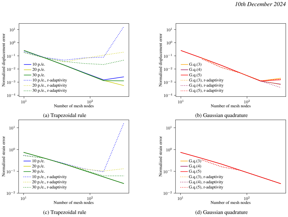
- [§4.2, Figure 9] The conclusion that Gaussian quadrature is more robust than the trapezoidal rule for r-adaptive meshes is based on a single run per configuration, and the reported data include a diverging case on the 10-node mesh and r-adaptive errors that are worse than fixed-mesh errors on several finer resolutions. Without repeated runs, error bars, or at least a statement about sensitivity to initialization and optimizer settings, the robustness comparison is not established. The authors should report variability over a few seeds or show that the observed behavior is deterministic by construction.
minor comments (5)
- [§3.2.2, Eq. (34)] Equation (34) appears to contain typos: the third column of the coordinate matrix should be the node c coordinates (xc, yc), but the text shows xb and yb twice.
- [§3.2.2, Eq. (41)] The expression for the physical coordinates of a quadrature point uses "ygi yaj + ygi ybj + ..." in the second component; this should presumably involve xg_i and yg_i as the barycentric coordinates for the x and y components, respectively.
- [§1] In the introduction, "we propose a new EFFEN framework named FENNI" should read "EFENN".
- [§3.2.2] The sentence "a propriety that will be used" should read "a property that will be used".
- [§3.2.3] The parameter controlling the maximum number of element splits is introduced in the methods text as "the maximal split value" but is not defined until Section 4.5, where it is set to 1; this should be specified when the refinement strategy is described.
Circularity Check
No significant circularity: FENNI's central claims are benchmarked against independent analytical and FEM reference solutions, and the only self-citations are motivational or implementation-related, not load-bearing.
full rationale
The paper's derivation chain is self-contained with respect to its claimed contributions. The FENNI architecture is built from standard reference-element shape functions and a sparse neural-network parameterization; the loss functions (potential energy, residual, weak form) are standard and are minimized without fitting any parameter to the reference solutions. The accuracy claims are assessed against an analytical solution in 1D and an independently computed fine-mesh FEM solution in 2D, so the results are not forced by construction. The h-adaptivity criterion in Eq. 43 is a heuristic based on relative Jacobian decrease, but it is not equivalent to the output it aims to improve; it is a methodological choice whose validity is tested empirically on the benchmark problems, not a fitted parameter disguised as a prediction. The multigrid training strategy initializes finer models from coarser trained models, and its speed-up is reported as measured computational time, not derived from the claim itself. Self-citations appear only as forward references to Part II for surrogate modeling, links to the authors' released code and demos, and a passing mention that a continuous equilibrium-gap formulation 'could be used here as well' (Genet, 2023); none of these carries the burden of the paper's central results. No uniqueness theorem is imported from prior work, and no ansatz is smuggled in via citation. The Jacobian-based refinement rule could be questioned as heuristic or insufficiently general, but that is a correctness/robustness concern, not circularity. Overall, the derivation and validation chain does not reduce to its own inputs.
Assumptions & free parameters
free parameters (5)
- h-adaptivity threshold tΔJ =
not stated
- residual loss weights λ1, λ2 =
λ1 = L, λ2 = 1
- maximum number of element splits =
1
- multigrid scaling factor =
2
- Gauss quadrature order =
1 point in 2D, 2 to 5 points in 1D
assumptions (5)
- standard math Reference-element shape functions and Gaussian quadrature provide a valid discretization for linear elastostatics.
- domain assumption Minimizing the potential energy or weak-form loss yields the solution of the strong-form PDE.
- ad hoc to paper The relative change of the Jacobian determinant identifies regions needing h-refinement.
- domain assumption A trained coarse-mesh solution is a good initialization for a finer mesh.
- domain assumption L-BFGS and Adam converge to a useful minimum of the nonconvex training loss.
Cite this review
Pith. "Pith review of Finite Element Neural Network Interpolation. Part I: Interpretable and Adaptive Discretization for Solving PDEs." pith.science (2026). https://pith.science/paper/EVEOY2SB
@misc{pith2026241205719,
  author       = {Pith},
  title        = {Pith review of: Finite Element Neural Network Interpolation. Part I: Interpretable and Adaptive Discretization for Solving PDEs},
  year         = {2026},
  howpublished = {\url{https://pith.science/paper/EVEOY2SB}},
  note         = {Machine review of arXiv:2412.05719}
}
read the original abstract
We present the Finite Element Neural Network Interpolation (FENNI) framework, a sparse neural network architecture extending previous work on Embedded Finite Element Neural Networks (EFENN) introduced with the Hierarchical Deep-learning Neural Networks (HiDeNN). Due to their mesh-based structure, EFENN requires significantly fewer trainable parameters than fully connected neural networks, with individual weights and biases having a clear interpretation. Our FENNI framework, within the EFENN framework, brings improvements to the HiDeNN approach. First, we propose a reference element-based architecture where shape functions are defined on a reference element, enabling variability in interpolation functions and straightforward use of Gaussian quadrature rules for evaluating the loss function. Second, we propose a pragmatic multigrid training strategy based on the framework's interpretability. Third, HiDeNN's combined rh-adaptivity is extended from 1D to 2D, with a new Jacobian-based criterion for adding nodes combining h- and r-adaptivity. From a deep learning perspective, adaptive mesh behavior through rh-adaptivity and the multigrid approach correspond to transfer learning, enabling FENNI to optimize the network's architecture dynamically during training. The framework's capabilities are demonstrated on 1D and 2D test cases, where its accuracy and computational cost are compared against an analytical solution and a classical FEM solver. On these cases, the multigrid training strategy drastically improves the training stage's efficiency and robustness. Finally, we introduce a variational loss within the EFENN framework, showing that it performs as well as energy-based losses and outperforms residual-based losses. This framework is extended to surrogate modeling over the parametric space in Part II.
Figures


Figures from the paper (12 more)




Forward citations
Cited by 1 Pith paper
-
Convex Neural Energy Elements: Monolithic Finite-Element Assembly of Geometry-Parameterized Neural Operators with Stability and Error Guarantees
Learning a convex element energy instead of a field turns one trained neural operator into reusable, geometry-parameterized finite elements with stability and error guarantees.
Reference graph
Works this paper leans on
-
[1]
& Martín, A
Badia, S., Li, W. & Martín, A. F. (2024). Finite element interpolated neural networks for solving forward and inverse problems. Computer Methods in Applied Mechanics and Engineering, 418, 116505 (cit. on p. 2). Berrone, S., Canuto, C. & Pintore, M. (2022a). Solving PDEs by variational physics-informed neural networks: An a posteriori error analysis. Annal...
2024
-
[2]
Cardiff, P. & Demirdži´c, I. (2021). Thirty Years of the Finite V olume Method for Solid Mechanics. Archives of Computational Methods in Engineering, 28(5), 3721–3780. https://doi.org/10.1007/s11831-020-09523-0 (cit. on p
-
[3]
Carstensen, C. (2004). An Adaptive Mesh-Refining Algorithm Allowing for an H1 Stable L2 Projection onto Courant Finite Element Spaces. Constructive Approximation, 20(4), 549–564. https://doi.org/10.1007/s00365-003- 0550-5 (cit. on p
-
[5]
Daby-Seesaram, A., Fau, A., Charbonnel, P.-É. & Néron, D. (2023). A hybrid frequency-temporal reduced-order method for nonlinear dynamics. Nonlinear Dynamics, 111(15), 13669–13689. https://doi.org/10.1007/s11071- 023-08513-8 (cit. on p
doi:10.1007/s11071- 2023
-
[6]
Daby-Seesaram, A., Škardová, K. & Genet, M. (2024a) . Finite Element Neural Network Interpolation: Part II - Hybridisation with the Proper Generalised Decomposition for non-linear surrogate modelling. Submitted (cit. on pp. 3, 22). Daby-Seesaram, A., Škardová, K. & Genet, M. (2024b) . NeuROM. https://doi.org/10.5281/zenodo.14218478. (Cit. on p
-
[8]
& Remacle, J
23 10th December 2024 Geuzaine, C. & Remacle, J. -F. (2020). A three-dimensional finite element mesh generator with built-in pre-and post-processing facilities. International Journal for Numerical Methods in Engineering, 11, 79 (cit. on p. 13). Khara, B., Balu, A., Joshi, A., Sarkar, S., Hegde, C., Krishnamurthy, A. & Ganapathysubramanian, B. (2024). Neuf...
2020
-
[9]
Liu, W. K., Li, S. & Park, H. S. (2022). Eighty Years of the Finite Element Method: Birth, Evolution, and Future. Archives of Computational Methods in Engineering, 29(6), 4431–4453. https://doi.org/10.1007/s11831-022- 09740-9 (cit. on p
-
[10]
Lu, Y., Blal, N. & Gravouil, A. (2018) . Multi-parametric space-time computational vademecum for parametric studies: Application to real time welding simulations. Finite Elements in Analysis and Design, 139, 62–72. https://doi.org/10.1016/j.finel.2017.10.008 (cit. on p
Show all 17 references
-
[11]
& Rønquist, E
Maday, Y. & Rønquist, E. M. (2002). A Reduced-Basis Element Method. Journal of Scientific Computing, 17(1), 447–459. https://doi.org/10.1023/A:1015197908587 (cit. on p
2002 doi
-
[12]
& Relun, N
Néron, D., Boucard, P.-A. & Relun, N. (2015). Time-space PGD for the rapid solution of 3D nonlinear parametrized problems in the many-query context. International Journal for Numerical Methods in Engineering, 103(4), 275–292. https://doi.org/10.1002/nme.4893 (cit. on p
2015 doi
-
[13]
Chatterjee, A. (2000). An introduction to the proper orthogonal decomposition. Current Science, 78(7), 808–817 (cit. on p. 2). Chinesta, F., Ladeveze, P. & Cueto, E. (2011) . A Short Review on Model Order Reduction Based on Proper Generalized Decomposition. Archives of Computa...
2000 doi
-
[14]
Du, H. & He, Q. (2024). Neural-integrated meshfree (nim) method: A differentiable programming-based hybrid solver for computational mechanics. Computer Methods in Applied Mechanics and Engineering, 427, 117024 (cit. on p. 2). Genet, M. (2023). Finite strain formulation of the ...
2024 doi
-
[15]
& Chinesta, F
Niroomandi, S., González, D., Alfaro, I., Bordeu, F., Leygue, A., Cueto, E. & Chinesta, F. (2013) . Real-time simulation of biological soft tissues: A PGD approach. International Journal for Numerical Methods in Biomedical Engineering, 29(5), 586–600. https://doi.org/10.1002/c...
2013 doi
-
[16]
Omella, Á. J. & Pardo, D. (2024) . R-adaptive deep learning method for solving partial differential equations. Computers & Mathematics with Applications, 153, 33–42 (cit. on p. 2). Penwarden, M., Zhe, S., Narayan, A. & Kirby, R. M. (2021) . Physics-informed neural networks (PI...
2024
-
[17]
& Karniadakis, G
Raissi, M., Perdikaris, P. & Karniadakis, G. E. (2019) . Physics-informed neural networks: A deep learning framework for solving forward and inverse problems involving nonlinear partial differential equations.Journal of Computational physics, 378, 686–707 (cit. on pp. 2, 5). S...
2019 doi
-
[18]
& Genet, M
Škardová, K., Daby-Seesaram, A. & Genet, M. (2024) . FENNI-I paper demo. https://doi.org/10.5281/zenodo. 14218368. (Cit. on p
2024 doi
-
[19]
& Srivastava, A
Sukumar, N. & Srivastava, A. (2022). Exact imposition of boundary conditions with distance functions in physics- informed deep neural networks. Computer Methods in Applied Mechanics and Engineering , 389, 114333 (cit. on p. 2). Wang, S., Teng, Y. & Perdikaris, P. (2021). Under...
2022
Reviewed August 11, 2026 · model on record in the stance chip above.
Discussion (0). Continue with ORCID to comment.