A decade of the fast-varying ionospheric and magnetospheric magnetic fields from ground and multi-satellite observations

Alexander Grayver; Jingtao Min

REVIEW 3 major objections 6 minor 12 references

A decade of the fast-varying ionospheric and magnetospheric magnetic fields from ground and multi-satellite observations

T0 review · 3 major / 6 minor · reviewed 2026-08-11 · deepseek-v4-flash

Challenge this review Re-run · record.json Download PDF Read on arXiv ↗ Review JSON

Pith's one-line read This paper claims that combined ground and satellite observations make the ionospheric–magnetospheric–induced field separation tractable, and demonstrates a 10-year, 3-hourly reconstruction.

desk verdict A genuinely new 10-year, 3-hourly product separating ionospheric, magnetospheric, and induced fields without temporal priors; the central thin-sheet assumption is under-validated but addressable, and the paper deserves a serious referee. read the letter →

arxiv 2412.10601 v2 pith:GEYQLENG submitted 2024-12-13 physics.space-ph physics.geo-ph

Jingtao Min , Alexander Grayver This is my paper · ORCID

classification physics.space-phphysics.geo-ph

keywords geomagneticfieldmodellingionosphericcurrentsmagnetosphericelectromagneticinductionsphericalharmonicanalysissatellitemagneticslunardailyvariationsstorms

verification ladder T0 review T1 audit T2 compute T3 formal

The pith

A machine-rendered reading of the paper's core claim, the machinery that carries it, and where it could break.

The reading

This paper tries to establish that the fast-varying magnetic fields of ionospheric, magnetospheric, and internally induced origin can be separated on a global scale when ground observatory data are combined with low-Earth-orbit satellite data. The key move is to treat the ionosphere as a thin current sheet, which gives a one-to-one relation between the fields it produces above and below the sheet, so the three sources map onto distinct spherical-harmonic coefficients. The authors estimate those coefficients independently in three-hour bins over 2014–2023, producing a continuous record that needs no assumed daily or seasonal rhythms. A reader should care because the separated record isolates storm-time ionospheric dynamics, links magnetospheric periodicities to solar rotation, and yields cleaner electromagnetic transfer functions for probing Earth's interior.

What carries the argument

The central object is the thin-sheet ionospheric model: a spherical current sheet of radius $a+h$ whose radial magnetic field is continuous. Equation (12) converts the ionospheric external coefficients into the internal coefficients seen from orbit, and substituting that relation into the two potential representations (13)–(14) reduces the unknowns to three independent sets of Gauss coefficients. This linear reparametrization is what makes the combined ground-satellite inversion tractable.

What would settle it

Apply the estimator to synthetic satellite and ground data generated from a three-dimensional ionospheric current model with vertical extent and field-aligned currents; if the thin-sheet assumption is load-bearing, the recovered magnetospheric coefficients will show ionospheric contamination, for example lunar tidal lines appearing in $q^\mathrm{mag}$.

Watch

Extended reading notes

Core claim

The paper claims that the internal/external ambiguity is broken by placing satellite observations between the ionosphere and the magnetosphere and modelling the ionosphere as a thin spherical sheet at radius $a+h$. The radial-field continuity condition $B_r|_{r\to(a+h)^+}=B_r|_{r\to(a+h)^-}$ gives a one-to-one link between the ionospheric external coefficients seen on the ground and the internal coefficients seen in orbit, so the potential can be rewritten with source-specific Gauss coefficients $(g^\mathrm{int}, q^\mathrm{ion}, q^\mathrm{mag})$ (Eqs. 13–14). Estimating these coefficients per three-hour bin over 2014–2023 yields a continuous, decade-long separation of the three sources.

Load-bearing premise

The load-bearing premise is that the ionosphere behaves as an infinitely thin current shell; if the real currents spread vertically or flow along magnetic field lines, the clean separation between the three sources fails.

Editorial extensions

If this is right

Because the parametrization imposes no time harmonics, the model can use day-side and storm-time data that most prior external-field models discard.
The 10-year coefficient series separates periodicities by source: lunar daily tidal lines appear in the ionospheric coefficients but not in the magnetospheric ones, a direct check on the separation.
Co-estimating the induced field yields C-responses with higher squared coherence and physically monotonic behavior at periods from 8 hours to 10 days, improving estimates used for mantle conductivity.
The three-hour time-binned construction can be updated as new low-latency data arrive, making it suitable for space-weather nowcasting.
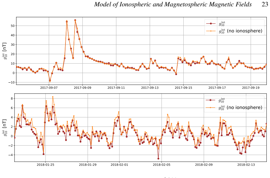
Storm-time reconstructions show the ionospheric equivalent current losing its quiet Sq vortex structure and developing transient high-latitude vortices, indicating the model captures non-periodic storm dynamics.

Reading between the lines

Editorial extensions of the paper, not claims the author makes directly.

The same geometric argument could be applied to other current layers, such as field-aligned currents, by exploiting observing shells at additional altitudes, provided each layer is thin enough for a sheet approximation.
Because the method needs no prior temporal harmonics, applying it to older satellite missions could extend the source-separated record backwards in time.
The three-hour bin width puts a floor on resolvable dynamics; substorm-scale events shorter than roughly three hours will be smoothed, so a denser satellite constellation would be the natural next test of how much faster the separation can go.
The co-estimated induced coefficients could be fed directly into 3-D mantle conductivity inversions, potentially replacing the quiet-time ionospheric corrections those inversions currently rely on.

Share X Bluesky LinkedIn Reddit HN

Signed reviews

No signed human review yet.

Editorial analysis

A structured set of objections, weighed in public.

Desk editor's note, referee report, and a circularity audit.

Desk Editor's Note

read the letter

The headline is simple: this paper delivers something that did not exist before — a decade-long, 3-hourly time series of separated ionospheric, magnetospheric, and induced Gauss coefficients, estimated with no prescribed temporal harmonics and across all local times and magnetic conditions. If the method holds up, it is a useful resource for storm-time external field studies and for mantle induction work. The core idea is sound: ground and satellite data combined with a thin-sheet ionosphere parametrization makes the three-way separation tractable, and the authors implement it carefully with cross-validated truncation, robust loss, and a sensible treatment of observatory biases (including a clear proof of the non-uniqueness in Appendix B). The validation is genuinely good. The qmag10 time series tracks CI and CHAOS during storms, lunar tidal peaks appear only in ionospheric coefficients and not in magnetospheric ones, and the Sq current vortices look right. The C-response comparison — with versus without an ionosphere — is a strong, physically meaningful check: co-modelling the ionosphere makes the transfer functions coherent and monotonic. That is real evidence the separation is working. The soft spots are real but not fatal. The biggest one is Eq. (12), the thin-sheet relation that ties ionospheric coefficients seen from the ground to those seen from satellites. It is load-bearing, yet the sheet height h is never stated, and no sensitivity test or direct validation of the relation is offered. Real ionospheric currents have vertical structure and field-aligned components, especially during storms, and if the relation is violated the inversion can leak ionospheric signal into the induced and magnetospheric coefficients. The authors should state h, test its influence, and justify the approximation against a finite-thickness or more realistic source. That is the main revision I would demand. Secondary issues: no uncertainty estimates for the coefficients, a uniform variance assumption that gets one sentence, no processing code, and several unresolved '??' figure references that make the manuscript feel unfinished. The abstract promises space weather nowcast/forecast benefits, but nothing in the paper demonstrates them; that sentence should be toned down or backed up. Overall, the mathematical structure is clear, the data product is new, and the internal checks are convincing enough that the work deserves refereeing. The thin-sheet concern is serious but addressable, and the rest is polish. I would send this to peer review and ask for a focused revision on h, uncertainties, and completeness. The likely audience — space physicists and EM induction modellers — will cite it if those issues are fixed.

Referee Report

3 major / 6 minor

Summary. The paper develops a new geomagnetic field modeling approach that simultaneously estimates mid-latitude ionospheric, magnetospheric, and internally induced magnetic fields by combining ground observatory and multi-satellite (Swarm, CryoSat-2, Grace-FO) vector data over 2014-2023. The method works in short (3-hour) time bins, imposes no temporal harmonic structure, and uses a thin-sheet approximation for ionospheric currents to link ground and satellite observations. Coefficients are estimated by robust least squares with model complexity selected via cross-validation. The resulting 10-year time series are analyzed in the frequency domain, revealing solar, lunar, and storm-time signatures, and are used to compute electromagnetic transfer functions (C-responses) that are more coherent and physically plausible when the ionosphere is explicitly modeled. The paper also demonstrates that omitting the ionosphere significantly biases induced-field estimates, especially at higher degrees.

Significance. If the separation is valid, this is a substantial methodological advance: it enables continuous, all-local-time, all-magnetic-condition monitoring of external and induced fields without prescribing temporal harmonics, which is relevant for space weather nowcasting and for electromagnetic induction studies. The paper provides several strong cross-checks: lunar tidal peaks appear only in ionospheric coefficients, the Sq current vortices are recovered with expected seasonal behavior, magnetospheric coefficients agree with CI and CHAOS models for the dominant modes, and the C-responses computed with the ionosphere included are smoother and more coherent. The availability of the coefficient time series on Zenodo and the use of cross-validation for model selection are also positive features. The main risk is that the central separation rests on an unquantified and unvalidated thin-sheet assumption for the ionosphere, and that no formal uncertainties accompany the coefficient time series.

major comments (3)

[Section 2, Eq. (12)] The thin-sheet relation (Eq. 12) is the only mechanism that connects the ionospheric field as seen by ground observatories (qion) and by satellites (gion), and it is therefore load-bearing for the central three-way separation claim. The manuscript does not state the numerical value of the sheet height h, nor does it provide any validation that the imposed radial Br continuity holds for the real ionosphere during the geomagnetic storms that the paper explicitly targets. Real ionospheric currents have finite vertical extent, field-aligned components, and day-night conductivity asymmetries, all of which violate Eq. (12) to some degree. I request that the authors: (i) specify h and justify the choice; (ii) perform a sensitivity analysis varying h over a plausible range (e.g., 90-120 km) and report how the separated coefficients change; and (iii) assess the error introduced by the thin-sheet approximation, for example by comparing against a model with a vertically extended ionospheric current layer or against independent ionospheric field estimates. Without such tests, the possibility that ionospheric signal leaks into the magnetospheric and induced coefficients through the parametrization in Eqs. (13)-(14) cannot be ruled out.
[Section 5.3 (and throughout)] The paper reports numerous spectral peaks (e.g., at 29.7, 27.0, 25.5 days; Rieger-type periods; lunar tidal lines) as robust features of the reconstructed fields, but no formal uncertainties are given for the estimated Gauss coefficient time series. Given that the separation depends on a structural assumption and that the data coverage changes over time (Fig. 3), it is important to know whether the claimed peaks are statistically significant. I ask the authors to provide at least approximate uncertainties, for example via bootstrap resampling of the time bins, jackknife estimates, or posterior covariances from the least-squares problem in each time bin, and to indicate the impact on the spectral interpretation.
[Section 3.2.1 and Appendix B] The observatory biases are estimated from a model that omits the ionosphere, under the argument that any static offset is small and does not affect temporal variability. However, the bias estimation is a separate regression on quiet-night data, and the resulting biases are then subtracted from the full dataset used in the main inversion. The sensitivity of the final separated coefficients to this preprocessing step is not quantified. Please provide a comparison of results obtained with the CI-derived biases versus the in-house biases, or a perturbation test that adds a plausible static offset to the biases and shows that the ionospheric, magnetospheric, and induced coefficient time series and the derived C-responses are materially unchanged.

minor comments (6)

[Equations (17) and (20)] The radical notation in Eq. (17) and the formatting of Eq. (20) are inconsistent and difficult to parse; please rewrite them in standard LaTeX style.
[Section 5.2, text near Figs. 7-10] There is a typo: "spacial" should be "spatial" in the sentence beginning "To get a glimpse of the spacial structure" (Section 6, first paragraph).
[Supplementary figures] The text contains several placeholder references such as "Fig. ??", "Table ??", and "Fig. ??" (e.g., Section 3.2.1 and Section 5.3). These need to be resolved to the actual supplementary figure and table numbers.
[Figures 4 and 5] The label "Kp 2" in the figure panels is ambiguous; it should read "Kp ≤ 2" for clarity, matching the text.
[Section 5.3] The statement "The uncertainty reported here is the resolution at the given peaks" applies to some but not all listed peak periods; please state the frequency resolution explicitly and apply it consistently to all quoted periods.
[Eq. (18) and Section 5.3] The lunar daily variation notation Lp is introduced with Eq. (18), but the index p is not defined (it is described in text as p=1,2,3,4). Please add the definition to the text preceding Eq. (18).

Circularity Check

0 steps flagged · score 2.0 of 10

No circular reduction: the ground–satellite separation rests on standard potential theory and an explicitly stated thin-sheet assumption, checked against independent benchmarks; self-citations are contextual only.

full rationale

The central derivation is self-contained and not circular. The paper's key step, Eq. (12), is a mathematical consequence of the explicitly stated thin-sheet assumption: 'assuming that the electric current in the ionosphere occupies a domain with limited radial extent, one can adopt the thin-sheet approximation... provides the continuity of the radial magnetic field across the thin sheet.' The one-to-one relation between qion and gion follows from Br continuity, not from fitting the desired output coefficients. The fact that the numerical value of h is not given is a model-assumption/robustness concern, not a circularity: an incorrect h would bias the estimates, but the derivation does not use the estimated ionospheric, magnetospheric, or induced coefficients to define the relation. The three-source coefficients are estimated by minimizing data misfit in each 3-hour bin, and the paper's validation relies on external benchmarks (CI and CHAOS models, known Sq morphology, lunar-period signatures appearing only in ionospheric coefficients, and physically monotonic C-responses) rather than on re-stating the model's own assumptions. Self-citations to prior work by Grayver and co-authors (e.g., Grayver et al. 2017, 2021, 2024; Kuvshinov et al. 2021) are contextual references for induction methodology and are not load-bearing for the present derivation. The appendices provide self-contained proofs of the bias non-uniqueness and the block-diagonal solver. No equation reduces by construction to a fitted parameter or to a self-citation chain, so no circular step is exhibited.

Assumptions & free parameters 7 free parameters · 7 assumptions · 0 invented entities

No new physical entities are introduced. The ionospheric thin-sheet and equivalent current streamfunction are standard representations, not new postulates. The free parameters are mostly data-processing choices (time bin, truncation, filters) plus the the ionospheric sheet height h, which is not quantified. The axioms are standard potential theory, the thin-sheet approximation, and assumptions about data errors and model subtraction accuracy.

free parameters (7)

Time bin duration = 3 hours
Chosen as a 'fair balance' between spatial and temporal resolution of the satellite data (Section 3). Non-overlapping bins define the temporal resolution of the model.
SH truncation degree for induced and magnetospheric fields = N = 4
Selected by 5-fold cross-validation and the Nyquist bound m<6 (Section 4); 25% more parameters in N=5 give only +0.002 in CV R2.
SH truncation degree for ionospheric field = N = 5
Chosen to capture Sq local-time structure while staying on the CV plateau (Section 4).
Ionospheric thin-sheet height h = not specified in the manuscript
Enters the ionosphere coupling relation Eq. (12); its value determines the amplitude of qion relative to gion, and no numerical value or literature source is given.
Quiet-time criteria for observatory bias estimation = Kp <= 2, |dDst/dt| <= 3 nT/h, solar elevation < -10 degrees
Thresholds used to select quiet-night data for bias estimation (Section 3.2.1); results depend on these choices.
Quasi-dipole latitude filter = 5 to 56 degrees
Data outside this mid-latitude band are discarded to exclude equatorial and polar electrojets (Section 3.1).
Huber loss robustness constant = not specified
A robust Huber loss is used for the inversion (Section 4), but the transition parameter is not given, affecting downweighting of outliers.

assumptions (7)

standard math The magnetic field in the region between the ionosphere and the magnetosphere is potential (MQS approximation), so it can be written as a gradient of a scalar potential satisfying Laplace's equation (Eqs. 1-4).
Used in Section 2 to justify the SH expansion.
domain assumption Ionospheric currents are confined to a thin spherical sheet at radius a+h, giving radial magnetic field continuity and the one-to-one relation between qion and gion (Eqs. 11-12).
Central to separating the three sources; the paper cites Sabaka et al. (2002) but does not state h.
domain assumption The CI core and lithospheric field models subtracted from the data are accurate enough that residuals are negligible for external-field estimation at degrees <=5.
Section 3.1 removes CI products; errors here alias directly into the estimated external coefficients.
domain assumption Magnetospheric and induced fields can be represented to SH degree 4 and the ionosphere to degree 5 with the available mid-latitude data, as chosen by CV and Nyquist arguments.
Section 4; higher-degree structure and local electrojets are unresolved by design.
domain assumption For the transfer-function analysis, the Earth responds as a radially symmetric (1-D) conductor to first order, so Qn depends only on degree n (Eq. 19).
Section 6; the authors argue 3-D effects are dwarfed by source effects.
domain assumption Observation errors are independent with uniform variance (W=I) within each bin.
Section 4; this neglects known differences between instruments and components and temporal correlations from 1-minute sampling.
domain assumption The omission of the ionosphere in the observatory-bias estimation only introduces a static offset because the nullspace of the joint problem is a static field.
Section 3.2.1 and Appendix B; used to justify the separate quiet-night bias estimation.

how reviews work

0 comments

Cite this review

Pith. "Pith review of A decade of the fast-varying ionospheric and magnetospheric magnetic fields from ground and multi-satellite observations." pith.science (2026). https://pith.science/paper/GEYQLENG

@misc{pith2026241210601,
  author       = {Pith},
  title        = {Pith review of: A decade of the fast-varying ionospheric and magnetospheric magnetic fields from ground and multi-satellite observations},
  year         = {2026},
  howpublished = {\url{https://pith.science/paper/GEYQLENG}},
  note         = {Machine review of arXiv:2412.10601}
}

read the original abstract

The time-varying geomagnetic field is a superposition of contributions from multiple internal and external current systems. A major source of geomagnetic variations at periods less than a few years are current systems external to the solid Earth, namely the ionospheric and magnetospheric currents, as well as associated induced currents. The separation of these three sources is mathematically underdetermined using either ground or satellite measurements alone, but becomes tractable when the two datasets are combined. Based on this concept, we developed a new geomagnetic field modelling approach that allows us to simultaneously characterise the mid-latitude ionospheric, magnetospheric and the internal induced magnetic fields using ground and satellite observations for all local times and magnetic conditions, and without prescribing any harmonic behaviour on these current systems in time, as is typical in other models. By applying this new method to a 10-year dataset of ground observatory and multi-satellite measurements from 2014 to 2023, we obtained the time series of the spherical harmonic coefficients of the ionospheric, magnetospheric and induced fields. These new time series allow the study of complex non-periodic dynamics of the external magnetic fields during global geomagnetic storms, as well as periodicities in the magnetospheric coefficients linked to solar activities and periodic ionospheric magnetic fields linked to lunar daily variations, contributing to a more complete picture of the dynamics of the external currents and magnetosphere-ionosphere interactions, and facilitating more accurate space weather nowcast and forecast. Finally, the new approach allows for a better characterisation of internal induced field sources, leading to higher quality electromagnetic transfer functions.

Figures

Figures reproduced from arXiv: 2412.10601 by the authors.

**Figure 1.** Geometric configuration of the model, showing time dependent spatially varying external and internal electric currents at middle geomagnetic latitudes (that is, excluding the polar regions). butions from electric currents induced in the Earth’s interior or in the ocean by nature of electromagnetic induction. We write these coefficients alternatively as g obs nm = g int nm, hobs nm = h int nm. (7) The satellite Gaus… view at source ↗

**Figure 2.** Distribution of ground observatories within 5 ◦N - 56◦N and 5 ◦S - 56◦S in magnetic latitude. The colour of the markers indicates the percentage of time bins where the observatory data are available in the period of 2013-2023. Since the spatial and temporal behaviour of the external field is of prime interest here, we impose no constraint on the magnetic conditions and inject no prior knowledge on the periodicity of… view at source ↗

**Figure 3.** Average number of data points per time bin as a function of time. Each vector component is treated as an independent datum. forward problem with the ionosphere is characterised by a static field. Therefore, the omission of the ionosphere in the bias estimation can only introduce a small static offset for the entire data span (10 years in our model), which does not interfere with the temporal variability of the field… view at source ↗

Figures from the paper (18 more)

**Figure 4.** Figure 4: The coefficient of determination R2 from fitting the whole ground observatory dataset (red) and from CV (blue) for models estimated using SH truncation degrees from 3 to 7. The square markers show the median of the R2 scores, while the upper and lower error bar limits …

**Figure 5.** Figure 5: Same as [PITH_FULL_IMAGE:figures/full_fig_p015_5.png]

**Figure 6.** Figure 6: Histogram of the coefficient of determination R2 based on the 5-fold cross-validation. the quality of the model and rule out the possibility of overfitting, we once again employ the CV approach. Using a 5-fold CV, we see that there is a drastic improvement in the CV av…

**Figure 7.** Figure 7: RMS difference for magnetospheric Gauss coefficients estimated using the models with and without the ionosphere. The rows show absolute (upper) and relative (lower) RMS differences, respectively. The columns show the RMS difference for the complete time series (left), …

**Figure 8.** Figure 8: 2-D histogram showing the distribution of the magnetospheric field Gauss coefficients estimated with and without the ionosphere layer in the model. The left panel shows the distribution for the P 0 1 mode, and the right panel shows the distribution for the P 1 2 mode. …

**Figure 9.** Figure 9: RMS difference for Gauss coefficients of the internally induced field estimated using the models with and without the ionosphere. The rows and columns are the same as in [PITH_FULL_IMAGE:figures/full_fig_p019_9.png]

**Figure 10.** Figure 10: 2-D histogram showing the distribution of the induced field Gauss coefficients estimated with and without ionosphere. The left panel shows the distribution for the P 0 1 mode, and the right panel shows the distribution for the P 1 2 mode. Lines show the linear fit to…

**Figure 11.** Figure 11: Time series of the magnetospheric Gauss coefficient q mag 10 (t) around the 2017 September geomagnetic storm (upper panel) and during magnetic quiet time, in January / February 2018 (lower panel). The plots show our model estimates (dark green lines), the estimates w…

**Figure 12.** Figure 12: Time series of the magnetospheric Gauss coefficient q mag 21 (t) around the 2017 September geomagnetic storm (upper panel) and during magnetic quiet time, in January / February 2018 (lower panel). external field model from the CI model (Sabaka et al. 2020) and the CH…

**Figure 13.** Figure 13: Time series of the ionospheric Gauss coefficient q ion 21 (t) around the 2017 September geomagnetic storm (upper panel) and during magnetic quiet time, in January / February 2018 (lower panel). field Gauss coefficients. The q ion 21 spatial mode ( [PITH_FULL_IMAGE:fi…

**Figure 14.** Figure 14: Time series of the internally induced Gauss coefficient g int 10 (t) around the 2017 September geomagnetic storm (upper panel) and during magnetic quiet time, in January / February 2018 (lower panel). The plots show our full model estimates (brown lines) and the esti…

**Figure 15.** Figure 15: Time series of the internally induced Gauss coefficient g int 21 (t) around the 2017 September geomagnetic storm (upper panel) and during magnetic quiet time, in January / February 2018 (lower panel). The first zonal harmonic of the magnetospheric magnetic field, lar…

**Figure 16.** Figure 16: Time series of the internally induced Gauss coefficient h int 32 (t) during magnetic quiet time, in February 2018 [PITH_FULL_IMAGE:figures/full_fig_p024_16.png]

**Figure 17.** Figure 17: Amplitude spectra of the magnetospheric coefficient q mag 10 (upper panel), the ionospheric coefficient q ion 10 coefficient (middle panel) and the internally induced coefficient g int 10 (lower panel). Spectral peaks observed in the spectra are marked with blue trian…

**Figure 18.** Figure 18: Amplitude spectra of the magnetospheric coefficient q mag 21 (upper panel), the ionospheric coefficient q ion 21 coefficient (middle panel) and the internally induced coefficient g int 21 (lower panel) around the diurnal band. Spectral peaks observed in the spectra ar…

**Figure 19.** Figure 19: Cn-responses (upper panel) and their squared coherences (lower panel) at periods between 8 hours and 10 days. The columns show the C1, C2, C3 and C4 responses estimated from the SH coefficients described by the P 0 1 , P 1 2 , P 2 3 and P 3 4 modes, respectively. ally…

**Figure 20.** Figure 20: Streamfunctions of the equivalent current for the ionospheric field (Ψion) on magnetic quiet days close to a spring equinox (left column) and a summer solstice (right column). The streamfunction is cut off above an absolute latitude of 70 degrees to filter out the val…

**Figure 21.** Figure 21: Streamfunction of the equivalent current for the ionospheric field (Ψion) during a geomagnetic storm on Sept. 8, 2017. The same cutoff latitude of 70 degrees is used. Note that the maximum value of the color scale is extended to twice of that for the quiet day plot ( …

Discussion (0). Continue with ORCID to comment.

Reference graph

Works this paper leans on

12 extracted references · 12 canonical work pages

[2]

1820–1980, Journal of Geophysical Research: Solid Earth , 94(B11), 15753–15769. Cane, H. V ., Richardson, I. G., & von Rosenvinge, T. T.,

work page 1980
[12]

(B.6) The nullity of the full system can be calculated via dim ker ( ~G⊤ ~G ) = dim ker (Nt∑ i=1 S⊤ i P⊥ GiSi ) ≥ rank(G′) = 1 3M0 (B.7) which concludes our proof that the problem has no unique least squares solution. From a physical point of view, when the complete model is augmented with observatory bias, an arbitrary time-invariant field can be embedde...

work page Pith review arXiv 2025
[1963]

Series A, Mathematical and Physical Sciences, 256(1066), 31–98

New methods for the analysis of geomagnetic fields and their application to the Sq field of 1932-3, Philosophical Transactions of the Royal Society of London. Series A, Mathematical and Physical Sciences, 256(1066), 31–98. Pulkkinen, A., Amm, O., & Viljanen, A.,

work page 1932
[1981]

Series A, Mathematical and Physical Sciences , 303(1473), 1–104

Spherical harmonic analysis of geomagnetic tides, 1964-1965,Philosophical Transactions of the Royal Society of London. Series A, Mathematical and Physical Sciences , 303(1473), 1–104. Winch, D. E., Ivers, D. J., Turner, J. P. R., & Stening, R. J.,

work page 1964
[1982]

Langlais, B

Some new methods in geomagnetic field modeling applied to the 1960-1980 epoch, Journal of Geomagnetism and Geoelectricity , 34(6), 327–349. Langlais, B. & Mandea, M.,

work page 1960
[1999]

methods, Geophysical Journal International , 136, 439–

A spherical harmonic analysis of solar daily variations in the years 1964-1965: Response 42 Min and Grayver estimates and source fields for global induction-I. methods, Geophysical Journal International , 136, 439–

work page 1964
[2000]

Larsson, J.,

An IGRF candidate main geomagnetic field model for epoch 2000 and a secular variation model for 2000–2005, Earth, Planets and Space , 52(12), 1137–1148. Larsson, J.,

work page 2000
[2005]

New parameterization of external and induced fields in geomag- netic field modeling, and a candidate model for IGRF 2005, Earth, Planets and Space ,

work page 2005

Show all 12 references

[2010]

Backus, G., Parker, R

A survey of cross-validation procedures for model selection, Statistics Surveys, 4, 40–79. Backus, G., Parker, R. L., & Constable, C., 1996.F oundations of Geomagnetism, Cambridge University Press. Baerenzung, J., Holschneider, M., Wicht, J., Lesur, V ., & Sanchez, S.,

1996
[2017]

Tsyganenko, N

Analysis of extreme solar activity in early September 2017: G4-severe geomagnetic storm (07-08.09) and GLE72 (10.09) in solar minimum, Comptes rendus de l’Acad ´emie bulgare des Sciences, 70(10), 1445–1456. Tsyganenko, N. A.,

2017
[2019]

The influence of geomagnetic storm of 7-8 September 2017 on the Swarm precise orbit determination, Journal of Geophysical Research: Space Physics, 124(8), 6971–6984. Model of Ionospheric and Magnetospheric Magnetic Fields 43 APPENDIX A: NON-UNIQUE LEAST SQUARES ESTIMATION OF A...

1982
[2024]

GFZ Data Services

Intermagnet Reference Data Set (IRDS) 2020 – Definitive Magnetic Observa- tory Data. GFZ Data Services. Juusola, L., Vanham¨aki, H., Viljanen, A., & Smirnov, M.,

2020

Pith tools

Reviewed August 11, 2026 · model on record in the stance chip above.

[1] [2]

1820–1980, Journal of Geophysical Research: Solid Earth , 94(B11), 15753–15769. Cane, H. V ., Richardson, I. G., & von Rosenvinge, T. T.,

work page 1980

[2] [12]

(B.6) The nullity of the full system can be calculated via dim ker ( ~G⊤ ~G ) = dim ker (Nt∑ i=1 S⊤ i P⊥ GiSi ) ≥ rank(G′) = 1 3M0 (B.7) which concludes our proof that the problem has no unique least squares solution. From a physical point of view, when the complete model is augmented with observatory bias, an arbitrary time-invariant field can be embedde...

work page Pith review arXiv 2025

[3] [1963]

Series A, Mathematical and Physical Sciences, 256(1066), 31–98

New methods for the analysis of geomagnetic fields and their application to the Sq field of 1932-3, Philosophical Transactions of the Royal Society of London. Series A, Mathematical and Physical Sciences, 256(1066), 31–98. Pulkkinen, A., Amm, O., & Viljanen, A.,

work page 1932

[4] [1981]

Series A, Mathematical and Physical Sciences , 303(1473), 1–104

Spherical harmonic analysis of geomagnetic tides, 1964-1965,Philosophical Transactions of the Royal Society of London. Series A, Mathematical and Physical Sciences , 303(1473), 1–104. Winch, D. E., Ivers, D. J., Turner, J. P. R., & Stening, R. J.,

work page 1964

[5] [1982]

Langlais, B

Some new methods in geomagnetic field modeling applied to the 1960-1980 epoch, Journal of Geomagnetism and Geoelectricity , 34(6), 327–349. Langlais, B. & Mandea, M.,

work page 1960

[6] [1999]

methods, Geophysical Journal International , 136, 439–

A spherical harmonic analysis of solar daily variations in the years 1964-1965: Response 42 Min and Grayver estimates and source fields for global induction-I. methods, Geophysical Journal International , 136, 439–

work page 1964

[7] [2000]

Larsson, J.,

An IGRF candidate main geomagnetic field model for epoch 2000 and a secular variation model for 2000–2005, Earth, Planets and Space , 52(12), 1137–1148. Larsson, J.,

work page 2000

[8] [2005]

New parameterization of external and induced fields in geomag- netic field modeling, and a candidate model for IGRF 2005, Earth, Planets and Space ,

work page 2005