REVIEW 2 major objections 6 minor 2 cited by
The Eclipsing Binaries via Artificial Intelligence. II. Need for Speed in PHOEBE Forward Models
T0 review · 2 major / 6 minor · reviewed 2026-08-11 · deepseek-v4-flash
Pith's one-line read A trained neural network surrogate for the PHOEBE binary-modeling code reproduces light curves with sub-percent error and runs MCMC sampling over 10,000 times faster.
desk verdict A solid, well-validated ANN surrogate for PHOEBE forward models within a restricted parameter box; the abstract overstates, but the core result is real and worth refereeing. read the letter →
The pith
A machine-rendered reading of the paper's core claim, the machinery that carries it, and where it could break.
The reading
What carries the argument
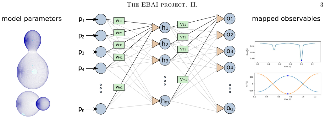
The load-bearing object is PHOEBAI, a fully connected feedforward ANN with six hidden layers of 512 nodes each, mapping six dimensionless eclipse-shape parameters ($e\sin\omega$, $e\cos\omega$, $\cos i$, $(R_1+R_2)/a$, $R_2/R_1$, $T_2/T_1$) to 501 normalized fluxes over orbital phases $-0.75$ to $0.25$. Once trained by regression on 1.25 million PHOEBE light curves (one million for training, 250,000 for validation), every forward evaluation is about $10^5$ cheap multiply-accumulate and activation operations—sub-millisecond—instead of PHOEBE's numerical surface discretization, atmosphere calls, and eclipse integration. The second piece of machinery is the dilution fraction $D = F_S/(F_S+F_B)$, applied after prediction as a flux-scaling parameter; including $D$ in the fit restores parameter recovery under light contamination.
What would settle it
Fit a set of detached eclipsing binaries with independently measured orbital and stellar parameters (from double-lined radial velocities and Gaia parallaxes) using PHOEBAI on their TESS light curves, and compare the recovered six parameters with the measured values; systematic mismatches above the claimed ~1% level, or accuracy collapsing for primaries outside the fixed F0 template, would falsify the surrogate's transfer claim.
Extended reading notes
Core claim
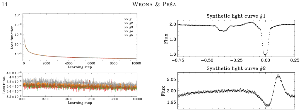
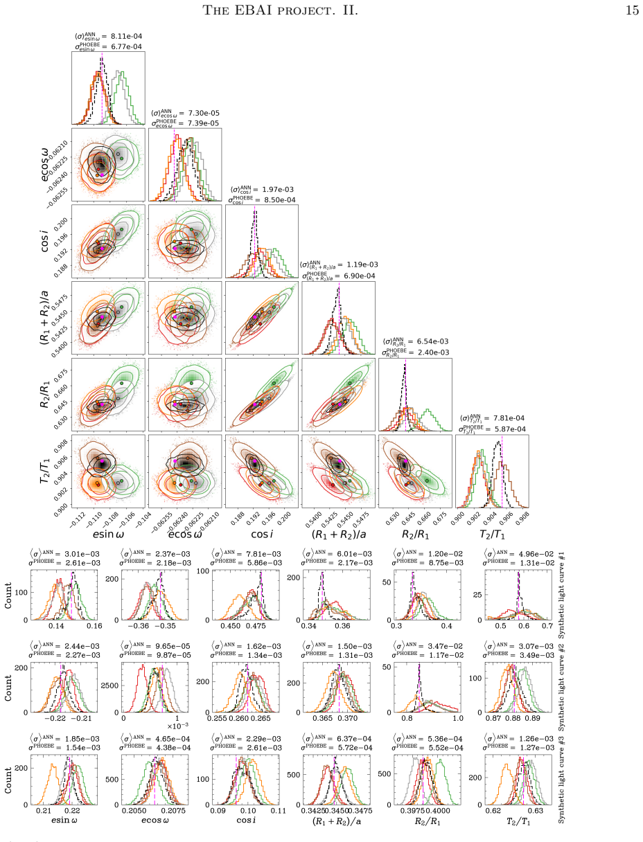
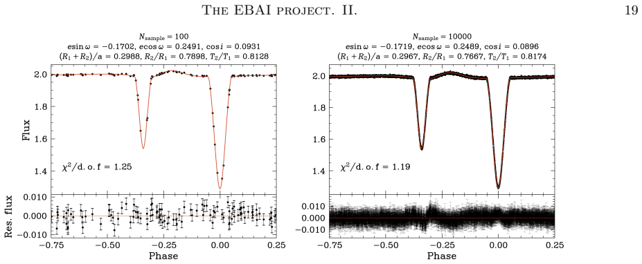
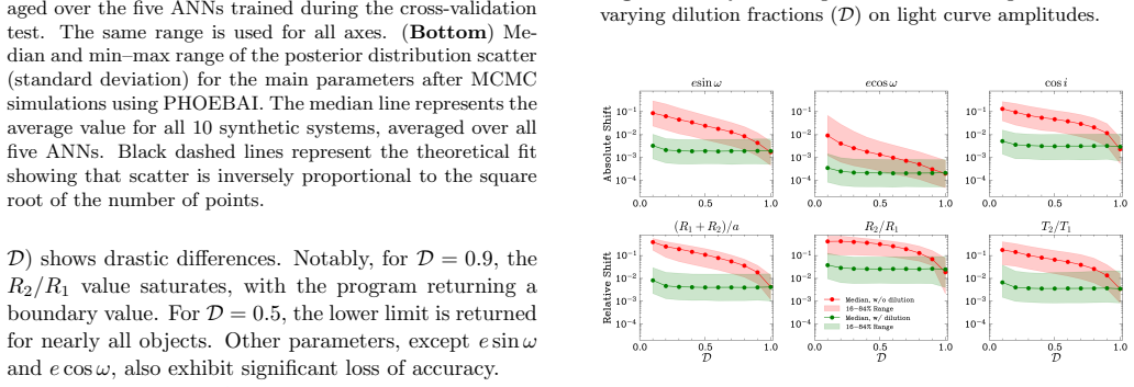
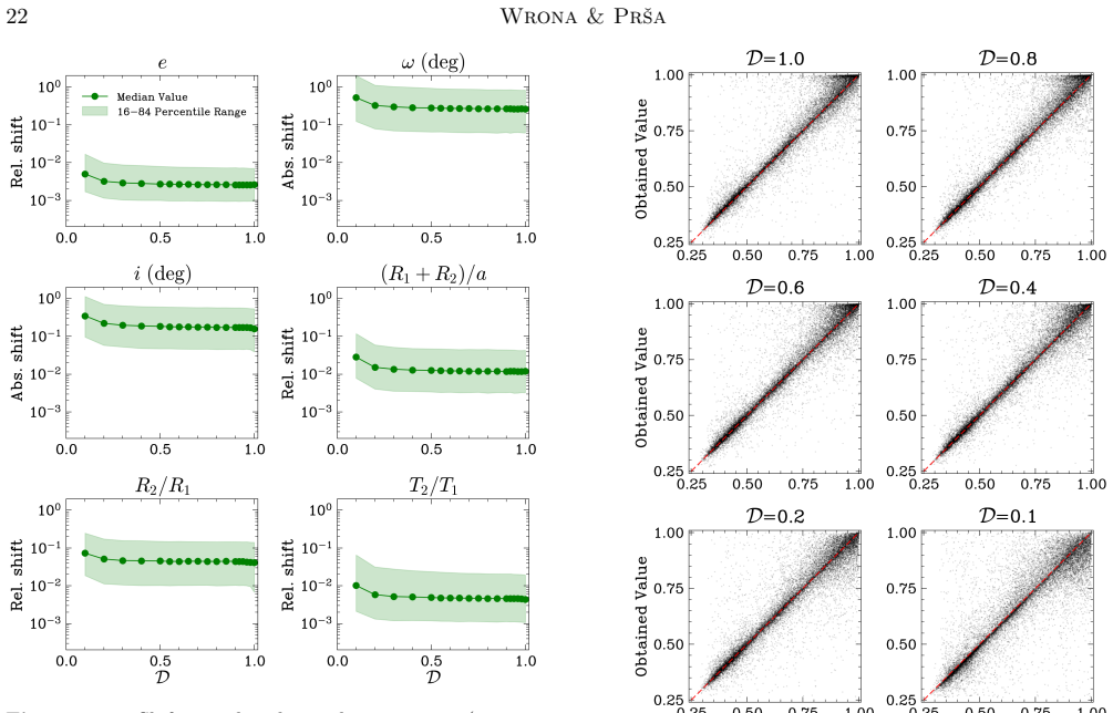
In the paper's own terms, a regression ANN can stand in for PHOEBE in the forward-model loop: feed it the six light-curve-shaping parameters—$e\sin\omega$, $e\cos\omega$, $\cos i$, $(R_1+R_2)/a$, $R_2/R_1$, and $T_2/T_1$—and it returns a 501-point phase-folded TESS light curve for a fixed F0 primary, with sub-percent systematic error across the training box. The chosen architecture, found by searching more than ten thousand configurations, has six hidden layers of 512 nodes with elu in the first hidden layer, sigmoid in the rest, a linear output, and the Adam optimizer. The claim is tested on synthetic data only: 100,000 unseen PHOEBE curves with realistic TESS noise are recovered with parameter accuracies around $10^{-3}$, the same behavior appears across five cross-validation networks, and the posterior distributions match PHOEBE's own sampling. The paper further claims that MCMC posterior scatter narrows as $N^{-1/2}$ with the number of data points while recovered parameter accuracy stays flat, so posterior width alone underestimates true uncertainty, and that adding a dilution fraction $D$ as a free parameter is necessary and sufficient to undo the bias that light contamination otherwise causes.
Load-bearing premise
The entire accuracy claim rests on PHOEBE's synthetic light curves being faithful stand-ins for real TESS observations of detached eclipsing binaries, so a network trained and tested only on PHOEBE output keeps its sub-percent errors when applied to nature.
Editorial extensions
If this is right
- A single CPU core can now produce MCMC posteriors for one detached EB in minutes rather than days, so population-scale studies of TESS, Kepler, and OGLE eclipsing binaries become computationally feasible.
- Because recovered parameter accuracy plateaus at the ANN's intrinsic noise near $10^{-3}$, collecting larger or higher-cadence light curves will not improve fitted parameters beyond that floor.
- MCMC posterior widths shrink as $N^{-1/2}$ even when accuracy is unchanged, so reported parameter error bars from sampling alone systematically overstate precision.
- Dilution must be included as a free parameter in AI-based EB fitting; without it, even weak contamination biases parameters substantially, with $R_2/R_1$ the most vulnerable.
- The surrogate only interpolates: optimization or sampling that leaves the training box invalidates the solution, so training sets must be kept complete and representative of real EB parameter distributions.
Reading between the lines
- The same six-layer architecture should transfer to other passbands and primary-star types by retraining on PHOEBE models; the limiting factor is the training distribution, not the network design.
- A practical extension would be to train directly on diluted light curves rather than adding $D$ post hoc, which could reduce the $D$ degeneracies the paper reports for uncontaminated systems.
- If the speedup survives contact with real data, catalog-scale reverse searches—fitting tens of thousands of systems to find rare configurations—become the natural next use of the surrogate.
- The posterior-scatter result implies that published EB uncertainties from MCMC alone are systematically underestimated; adding the surrogate's systematic floor in quadrature would make error bars honest.
Editorial analysis
A structured set of objections, weighed in public.
Referee Report
Summary. The paper presents PHOEBAI, a fully connected feedforward neural network trained on about 1.25 million PHOEBE-generated synthetic light curves to emulate the forward model for detached eclipsing binaries. The network maps six parameters (e sin ω, e cos ω, cos i, (R1+R2)/a, R2/R1, T2/T1) to a 501-point TESS-band light curve. The authors select a 6×512 architecture via a large hyperparameter search, then validate it with five-fold cross-validation, noise-injection studies spanning six decades of uncertainty, a held-out set of 100,000 systems, data-size scaling tests, and dilution studies with about 10,000 fits. They report a speedup of more than four orders of magnitude in MCMC sampling (2.16 s vs. 21.63 hr on the same hardware with identical sampler settings) and systematic parameter errors below 1%, often near 0.01%, within the training box. The paper also demonstrates that including a dilution fraction as a free parameter is essential for accurate parameter recovery when light contamination is present.
Significance. If the reported accuracy and speed hold, PHOEBAI is a practical drop-in surrogate for PHOEBE in optimization and MCMC sampling for the six-parameter detached-EB problem, enabling population-scale analyses that are currently prohibitively expensive. The paper's strengths are its extensive internal validation: five-fold cross-validation with five independently trained networks, noise injection over six decades, 100,000 unseen systems, data-size scaling, and roughly 10,000 dilution fits. The timing comparison is concrete and fair, using identical sampler settings and hardware. The paper also honestly discusses limitations, notably in Section 6, where it states that additional networks must be trained for different primary stars and passbands. The main caveat is that the accuracy claims are validated only on synthetic light curves drawn from the same filtered, fixed-primary, TESS training distribution, so the headline 'entire parameter space' claim needs to be scoped accordingly.
major comments (2)
- [Abstract and Section 5.1] The abstract's claim of 'systematic errors not exceeding 1% ... across the entire parameter space' is not supported as stated. The network is trained and tested with the primary fixed to M1=1.61 Msun, R1=1.728 Rsun, T1=7220 K (Section 5.1), a single passband (TESS T, Section 4.2), and a filtered parameter distribution that enforces R2<=R1, T2<=T1, eclipse amplitude >0.01, and no Roche-lobe overflow. The 'entire parameter space' is therefore the filtered, fixed-primary, TESS training box, not the space of real eclipsing binaries. The sentence in Section 5.1 that fixing the primary 'does not cause any loss of generality' is an unsupported assertion; Section 6 correctly acknowledges that new networks are needed for different primaries. Please revise the abstract and conclusions to state 'within the parameter space used for training' and remove or substantially qualify the 'no loss of generality' sentence.
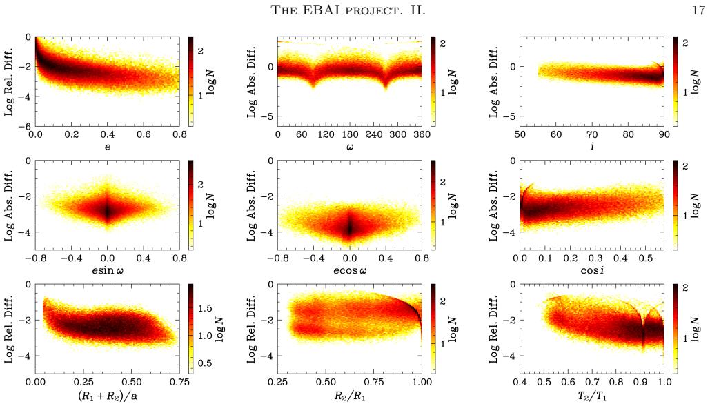
- [Section 5.3.2, Table 3, and Section 6] The errors reported in Table 3 and described in Section 6 as 'systematic errors' are end-to-end parameter-recovery errors on synthetic data. They include the ANN approximation error, the optimizer/sampler's ability to find the best model, parameter degeneracies, and the effect of edge-of-range solutions. The paper never reports a direct comparison of ANN-predicted fluxes against PHOEBE fluxes on a held-out set, so the 'intrinsic noise' level of the ANN is inferred rather than measured. Please clarify in the text that Table 3 quantifies the total recovery floor, not the ANN forward-model error alone, and state whether direct flux-level metrics (e.g., MSE or MedAE on the held-out set) were computed; if they were, reporting them would strengthen the paper, and if not, the systematic-error language should be qualified accordingly.
minor comments (6)
- [Section 5.4] The dilution model is described verbally but no equation is given for how the ANN-predicted light curve is modified when D is a free parameter. A formula such as F_obs = D * F_ann + (1-D) * B, or the equivalent, would remove ambiguity about whether D multiplies the entire ANN output or acts on the variability amplitude.
- [Section 4.1] The rule of thumb '10 per degree of freedom' is said to imply a sample size of about one million for six parameters, but 10 per degree of freedom would give 60. This sentence is confusing and should be reworded or corrected, perhaps by clarifying that the one-million figure comes from the required density and nonlinearity of the mapping rather than this simple rule.
- [Table 3] Table 3 mixes absolute errors (e sin ω, e cos ω, cos i) and relative errors ((R1+R2)/a, R2/R1, T2/T1) without stating this in the caption. Please specify which columns are absolute and which are relative to avoid misinterpretation of the '1%' claim.
- [Section 5.3.1] The cross-validation description says 'five equal parts (validation sets)' but then states each training set has one million entries and each validation set has 250,000. Please clarify that the five validation sets are disjoint 250,000-entry subsets of the 1.25 million dataset, with the remaining one million used for training in each fold.
- [Figure 15] The lower panel shows fitted lines of the form A/sqrt(N) for the posterior scatter, but the fit parameters A and any uncertainties are not reported. Adding the fitted values would let readers reproduce the scaling claim.
- [References] The reference list contains a duplicate entry for Virtanen et al. 2020. Please remove the duplication.
Circularity Check
No significant circularity: PHOEBAI is a standard, internally consistent emulator of PHOEBE validated on held-out synthetic light curves; the abstract's scope is narrower than its wording, but that is a generalization limitation, not circularity.
full rationale
The paper's central claim is that a fixed 6x512 feedforward ANN can reproduce PHOEBE forward models for detached eclipsing binaries in the six-parameter training box, with a >10^4 speedup and ~1e-3-level parameter recovery on synthetic data. This claim is not circular: the ANN is a supervised regression emulator, and its accuracy is tested on 100,000 held-out PHOEBE light curves never used in training, plus five-fold cross-validation (Secs. 5.3.1, 5.3.3). The 'systematic errors' are emulator approximation and inversion errors relative to known synthetic truth, not astrophysical validation; Table 3 and Sec. 6 characterize the intrinsic noise floor of ~1e-3 and state that new networks are needed for other primaries and passbands. The speedup is measured directly with identical samplers and hardware (Sec. 6). The paper explicitly discloses the fixed F0 primary (M1=1.61 Msun, R1=1.728 Rsun, T1=7220 K, Sec. 5.1) and the single TESS band (Sec. 4.2), so the abstract's 'entire parameter space' is the filtered training box; this is an overstatement of scope but does not make the derivation self-referential. The only self-citations (Prsa et al. 2008 for the parameter set, Prsa et al. 2022 for TESS noise) are contextual and not load-bearing: the surrogate's performance does not rest on those citations being true. No equation is defined in terms of the quantity it purports to predict, and no fitted parameter is renamed as a prediction. The emulator accuracy is genuinely evaluated on inputs outside the training set, even though those inputs share the same generator; that is standard surrogate validation, not circularity. Transfer to real observations is an open limitation, not a circular step.
Assumptions & free parameters
free parameters (3)
- Training-set parameter distributions =
e ~ U(0,0.8); cos i ~ U(cos 90, cos 55); (R1+R2)/a ~ U(0.04,0.75); M2 ~ U(0.59,1.61) Msun; log-normal spreads 0.075…
- Fixed primary stellar parameters =
M1=1.61 Msun, R1=1.728 Rsun, T1=7220 K
- Low-noise threshold for reporting systematic errors =
sigma <= 1e-3 in relative flux
assumptions (3)
- domain assumption PHOEBE 2.4.16 is a faithful forward model for detached eclipsing binary light curves in the TESS band, including Roche geometry, Castelli & Kurucz atmospheres, gravity darkening, and reflection.
- domain assumption The sampled parameter distributions (based on Raghavan et al. 2010, Duchene & Kraus 2013, Moe & Di Stefano 2017, Pecaut & Mamajek 2013) are representative of the real detached EB population, and interpolation within the filtered training box is sufficient.
- ad hoc to paper Exclusion filters (eclipse amplitude > 0.01, no Roche lobe overflow, R2 <= R1, T2 <= T1) define a physically valid but biased subset of the parameter space; the ANN is validated only on this filtered subset.
Cite this review
Pith. "Pith review of The Eclipsing Binaries via Artificial Intelligence. II. Need for Speed in PHOEBE Forward Models." pith.science (2026). https://pith.science/paper/BHCMPQNG
@misc{pith2026241211837,
  author       = {Pith},
  title        = {Pith review of: The Eclipsing Binaries via Artificial Intelligence. II. Need for Speed in PHOEBE Forward Models},
  year         = {2026},
  howpublished = {\url{https://pith.science/paper/BHCMPQNG}},
  note         = {Machine review of arXiv:2412.11837}
}
read the original abstract
In modern astronomy, the quantity of data collected has vastly exceeded the capacity for manual analysis, necessitating the use of advanced artificial intelligence (AI) techniques to assist scientists with the most labor-intensive tasks. AI can optimize simulation codes where computational bottlenecks arise from the time required to generate forward models. One such example is PHOEBE, a modeling code for eclipsing binaries (EBs), where simulating individual systems is feasible, but analyzing observables for extensive parameter combinations is highly time-consuming. To address this, we present a fully connected feedforward artificial neural network (ANN) trained on a dataset of over one million synthetic light curves generated with PHOEBE. Optimization of the ANN architecture yielded a model with six hidden layers, each containing 512 nodes, provides an optimized balance between accuracy and computational complexity. Extensive testing enabled us to establish ANN's applicability limits and to quantify the systematic and statistical errors associated with using such networks for EB analysis. Our findings demonstrate the critical role of dilution effects in parameter estimation for EBs, and we outline methods to incorporate these effects in AI-based models. This proposed ANN framework enables a speedup of over four orders of magnitude compared to traditional methods, with systematic errors not exceeding 1\%, and often as low as 0.01\%, across the entire parameter space.
Figures


Figures from the paper (16 more)







Forward citations
Cited by 2 Pith papers
-
The present and the future of modeling eclipsing binary systems
A review of eclipsing binary modeling argues for separate boutique and bulk approaches and demonstrates a neural-network emulator that runs much faster than the physical model.
-
From stellar light to astrophysical insight: automating variable star research with machine learning
An invited review of machine learning for automated variable star research, covering data cleaning, variability classification, stellar parameter inference, and foundation models.
Reference graph
Works this paper leans on
-
[1]
Intrinsic Colors, Temperatures, and Bolometric Corrections of Pre-main-sequence Stars
thebibliography [1] 20pt to REFERENCES 6pt =0pt -12pt 10pt plus 3pt =0pt =0pt =1pt plus 1pt =0pt =0pt -12pt =13pt plus 1pt =20pt =13pt plus 1pt \@M =10000 =-1.0em =0pt =0pt 0pt =0pt =1.0em @enumiv\@empty 10000 10000 `\.\@m \@noitemerr \@latex@warning Empty `thebibliography' environment \@ifnextchar \@reference \@latexerr Missing key on reference command E...
-
[2]
2015, TensorFlow : Large-Scale Machine Learning on Heterogeneous Systems
Abadi, M., Agarwal, A., Barham, P., et al. 2015, TensorFlow : Large-Scale Machine Learning on Heterogeneous Systems. https://www.tensorflow.org/
2015
-
[3]
2011, in American Institute of Physics Conference Series, Vol
Arenou , F. 2011, in American Institute of Physics Conference Series, Vol. 1346, American Institute of Physics Conference Series, ed. J. A. Docobo , V. S. Tamazian , & Y. Y. Balega , 107--121, 10.1063/1.3597593
-
[4]
Astropy Collaboration , Price-Whelan , A. M., Sip o cz , B. M., et al. 2018, , 156, 123, 10.3847/1538-3881/aabc4f
-
[5]
Bailer-Jones , C. A. L., Rybizki , J., Fouesneau , M., Mantelet , G., & Andrae , R. 2018, , 156, 58, 10.3847/1538-3881/aacb21
-
[6]
2019, Canadian Association of Radiologists Journal, 70, 344, 10.1016/j.carj.2019.06.002
Balki, I., Amirabadi, A., Levman, J., et al. 2019, Canadian Association of Radiologists Journal, 70, 344, 10.1016/j.carj.2019.06.002
-
[7]
Barclay , T., Huber , D., Rowe , J. F., et al. 2012, , 761, 53, 10.1088/0004-637X/761/1/53
-
[8]
J., Koch , D., Basri , G., et al
Borucki , W. J., Koch , D., Basri , G., et al. 2010, Science, 327, 977, 10.1126/science.1185402
Show all 50 references
-
[9]
Castelli , F., & Kurucz , R. L. 2004, ArXiv Astrophysics e-prints
2004
-
[10]
2015, Keras, https://keras.io
Chollet, F., et al. 2015, Keras, https://keras.io
2015
-
[11]
2011, , 529, A75, 10.1051/0004-6361/201116451
Claret , A., & Bloemen , S. 2011, , 529, A75, 10.1051/0004-6361/201116451
2011 doi
-
[12]
E., Pr s a , A., Stassun , K
Conroy , K. E., Pr s a , A., Stassun , K. G., et al. 2014, , 147, 45, 10.1088/0004-6256/147/2/45
2014 doi
-
[13]
E., Kochoska , A., Hey , D., et al
Conroy , K. E., Kochoska , A., Hey , D., et al. 2020, , 250, 34, 10.3847/1538-4365/abb4e2
2020 doi
-
[14]
2023, Gaia Data Release Scenario, https://www.cosmos.esa.int/web/gaia/release
Consortium, G. 2023, Gaia Data Release Scenario, https://www.cosmos.esa.int/web/gaia/release
2023
-
[15]
2013, , 51, 269, 10.1146/annurev-astro-081710-102602
Duch \^e ne , G., & Kraus , A. 2013, , 51, 269, 10.1146/annurev-astro-081710-102602
2013 doi
-
[16]
2017, , 154, 220, 10.3847/1538-3881/aa9332
Foreman-Mackey , D., Agol , E., Ambikasaran , S., & Angus , R. 2017, , 154, 220, 10.3847/1538-3881/aa9332
2017 doi
-
[17]
W., Lang , D., & Goodman , J
Foreman-Mackey , D., Hogg , D. W., Lang , D., & Goodman , J. 2013, , 125, 306, 10.1086/670067
2013 doi
-
[18]
A., & Skapura, D
Freeman, J. A., & Skapura, D. M. 1991, Neural networks: algorithms, applications, and programming techniques (Redwood City, CA, USA: Addison Wesley Longman Publishing Co., Inc.)
1991
-
[19]
Gaia Collaboration , Brown , A. G. A., Vallenari , A., et al. 2021, , 649, A1, 10.1051/0004-6361/202039657
2021 doi
-
[20]
2010, Communications in Applied Mathematics and Computational Science, 5, 65, 10.2140/camcos.2010.5.65
Goodman , J., & Weare , J. 2010, Communications in Applied Mathematics and Computational Science, 5, 65, 10.2140/camcos.2010.5.65
2010 doi
-
[21]
M., Kurtz , D
Hambleton , K. M., Kurtz , D. W., Pr s a , A., et al. 2013, , 434, 925, 10.1093/mnras/stt886
2013 doi
-
[22]
2015, in Astrophysics and Space Science Library, Vol
Huber , D. 2015, in Astrophysics and Space Science Library, Vol. 408, Giants of Eclipse: The Aurigae Stars and Other Binary Systems, 169, 10.1007/978-3-319-09198-3_7
2015 doi
-
[23]
Hunter , J. D. 2007, Computing in Science and Engineering, 9, 90, 10.1109/MCSE.2007.55
2007 doi
-
[24]
Lucy , L. B. 1967, , 65, 89
1967
-
[25]
Luri , X., Brown , A. G. A., Sarro , L. M., et al. 2018, , 616, A9, 10.1051/0004-6361/201832964
2018 doi
-
[26]
2017, , 230, 15, 10.3847/1538-4365/aa6fb6
Moe , M., & Di Stefano , R. 2017, , 230, 15, 10.3847/1538-4365/aa6fb6
2017 doi
-
[27]
Oliphant, T. E. 2006, A guide to NumPy, Vol. 1 (Trelgol Publishing USA)
2006
-
[28]
Orosz , J. A. 2015, in Astronomical Society of the Pacific Conference Series, Vol. 496, Living Together: Planets, Host Stars and Binaries, ed. S. M. Rucinski , G. Torres , & M. Zejda , 55. 1503.07295
2015 arXiv
-
[29]
J., & Mamajek , E
Pecaut , M. J., & Mamajek , E. E. 2013, , 208, 9, 10.1088/0067-0049/208/1/9
2013 doi
-
[30]
2011, Journal of Machine Learning Research, 12, 2825
Pedregosa, F., Varoquaux, G., Gramfort, A., et al. 2011, Journal of Machine Learning Research, 12, 2825
2011
-
[31]
F., Devinney , E
Pr s a , A., Guinan , E. F., Devinney , E. J., et al. 2008, , 687, 542, 10.1086/591783
2008 doi
-
[32]
2005, , 628, 426, 10.1086/430591
Pr s a , A., & Zwitter , T. 2005, , 628, 426, 10.1086/430591
2005 doi
-
[33]
2018, Modeling and Analysis of Eclipsing Binary Stars; The theory and design principles of PHOEBE (Institute of Physics), 10.1088/978-0-7503-1287-5
Pr s a , A. 2018, Modeling and Analysis of Eclipsing Binary Stars; The theory and design principles of PHOEBE (Institute of Physics), 10.1088/978-0-7503-1287-5
2018 doi
-
[34]
2019, , 131, 068001, 10.1088/1538-3873/ab0f41
Pr s a , A., Zhang , M., & Wells , M. 2019, , 131, 068001, 10.1088/1538-3873/ab0f41
2019 doi
-
[35]
E., et al
Pr s a , A., Kochoska , A., Conroy , K. E., et al. 2022, , 258, 16, 10.3847/1538-4365/ac324a
2022 doi
-
[36]
A., Henry , T
Raghavan , D., McAlister , H. A., Henry , T. J., et al. 2010, , 190, 1, 10.1088/0067-0049/190/1/1
2010 doi
-
[37]
R., Winn , J
Ricker , G. R., Winn , J. N., Vanderspek , R., et al. 2015, Journal of Astronomical Telescopes, Instruments, and Systems, 1, 014003, 10.1117/1.JATIS.1.1.014003
2015 doi
- [38]
-
[39]
2022, in Artificial Intelligence, ed
Roy, S., & Dubey, J. 2022, in Artificial Intelligence, ed. A. A. Sk, T. Turki, T. K. Ghosh, S. Joardar, & S. Barman (Cham: Springer Nature Switzerland), 191--201
2022
-
[40]
Russell , H. N. 1948, in Harvard Observatory Monographs, Vol. 7 (Harvard Observatory), 181
1948
-
[41]
W., Pr s a , A., Welsh , W
Slawson , R. W., Pr s a , A., Welsh , W. F., et al. 2011, , 142, 160, 10.1088/0004-6256/142/5/160
2011 doi
-
[42]
2014, , 147, 86, 10.1088/0004-6256/147/4/86
Tokovinin , A. 2014, , 147, 86, 10.1088/0004-6256/147/4/86
2014 doi
-
[43]
2010, , 18, 67, 10.1007/s00159-009-0025-1
Torres , G., Andersen , J., & Gim \'e nez , A. 2010, , 18, 67, 10.1007/s00159-009-0025-1
2010 doi
-
[45]
E., et al
Virtanen , P., Gommers , R., Oliphant , T. E., et al. 2020, Nature Methods, 17, 261, https://doi.org/10.1038/s41592-019-0686-2
2020 doi
-
[46]
Vogt , F. P. A., Bond , H. E., Cracraft , M. M., et al. 2014, in American Astronomical Society Meeting Abstracts, Vol. 223, American Astronomical Society Meeting Abstracts \#223, 154.18
2014
-
[47]
2017, , 129, 065003, 10.1088/1538-3873/aa682a
Wells , M., Pr s a , A., Jones , L., & Yoachim , P. 2017, , 129, 065003, 10.1088/1538-3873/aa682a
2017 doi
- [48]
-
[49]
F., Orosz , J
Welsh , W. F., Orosz , J. A., Short , D. R., et al. 2015, , 809, 26, 10.1088/0004-637X/809/1/26
2015 doi
-
[50]
Wilson , R. E. 1990, , 356, 613, 10.1086/168867
1990 doi
- [51]
Reviewed August 11, 2026 · model on record in the stance chip above.
Discussion (0). Continue with ORCID to comment.