REVIEW 2 major objections 4 minor 55 references
The Line operators in the G2HDM model
T0 review · 2 major / 4 minor · reviewed 2026-08-11 · deepseek-v4-flash
Pith's one-line read The paper argues that the discrete center quotient $\Gamma$ of the G2HDM gauge group — invisible to local experiments — determines the spectra of Wilson, 't Hooft, and dyonic line operators, the periodicity of the five CP-violating…
desk verdict Solid extension of Tong's line-operator program to G2HDM, but the mixed U(1)_V/U(1)_A section drops the charge-lattice parity constraint and overcounts spectra. read the letter →
The pith
A machine-rendered reading of the paper's core claim, the machinery that carries it, and where it could break.
The reading
What carries the argument
The engine is the generalized Dirac quantization condition, Eq. (18) (with the $U(1)_V\times U(1)_A$ version in Eq. (26)), read as a mod-6 constraint on pairs of electric and magnetic labels: $(z_e^2,z_e^3,q; z_m^2,z_m^3,g)$ for the visible factor and $(x_e^2,h; x_m^2,k)$ for the dark factor. Quotienting by $\Gamma$ is implemented by demanding invariance of Wilson lines under the quotient generators, which restricts the electric weights; the magnetic spectrum is then solved from the quantization condition. For the $\theta$-angles the machinery is the combined $U(1)\times SU(N)\times SU(M)$ $\theta$-term of Eq. (31), from which the periodicities and CP-invariant values are read off; for symmetry breaking it is the Gell-Mann-Nishijima-style formulas $Q_{\rm em}=q/6+\lambda_e^2/2$ and $Q_D=h/2+\rho_e^2/2$ together with the deconfinement conditions $6g\equiv z_m^2 \pmod 2$ and $2k\equiv x_m^2 \pmod 2$.
What would settle it
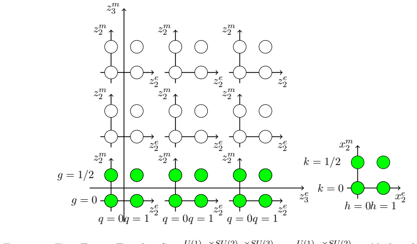
Compute the full set of allowed line operators for one quotient, say $G = (U(1)_Y\times SU(2)_L\times SU(3)_C)/Z_{6L} \times (U(1)_X\times SU(2)_H)/1$, directly from the weight and co-weight lattices of the covering group without importing Eq. (18) as an axiom; if the resulting lattice differs from the paper's Fig. 8, the spectra change. Experimentally, discover a magnetic monopole and measure whether it satisfies the electromagnetic Dirac condition for leptons but not for quarks: the paper predicts the quotient must then contain $Z_{6L}$ or $Z_{6H}$, so a monopole with exactly the opposite pattern would falsify the central claim.
Extended reading notes
Core claim
The central claim is that the G2HDM's global gauge structure is not invisible: the discrete quotient $\Gamma$ changes the lattice of allowed non-local operators and the topological angles attached to them. Concretely, for each quotient pattern the allowed Wilson and 't Hooft lines are the subsets of the covering-group lattices left invariant by $\Gamma$, with coexisting dyonic lines constrained by the generalized Dirac quantization condition $-6gq + 3z_e^2 z_m^2 + 2z_e^3 z_m^3 + 3x_e^2 x_m^2 - 6kh \equiv 0 \pmod 6$ (and its $U(1)_V \times U(1)_A$ variant). The same data determine the $\theta$-angle periodicities, which range from $2\pi$ up to $72\pi$ for $\tilde\theta_Y$ and $8\pi$ for $\tilde\theta_X$ depending on $\Gamma$. After the two-step breaking $SU(2)_H \times U(1)_X \to U(1)_D$ and $SU(2)_L \times U(1)_Y \to U(1)_{\rm em}$, the minimal charges shift: for instance $Q_{\rm em}$ can be $1/6$, $1/3$, or $1/2$, with magnetic counterpart $G_{\rm em}$ equal to $1$, $2$, $3$, or $6$. When $\Gamma$ contains the $SU(3)_C$ center, the minimal electromagnetic monopole violates the pure Dirac condition and must carry color magnetic charge, so the low-energy group becomes $U(3)_C$; when the mixed $U(1)_V \times U(1)_A$ basis is quotiented by $Z_{2L}\times Z_{2H}$ or $Z_{6L}\times Z_{2H}$, even the dark Dirac condition can fail. The paper also identifies the residual dark QED angle $\theta_{\rm dem} = (\tilde\theta_X + 2\theta_{2H})/4$ as the physical, chiral-rotation-invariant counterpart of $\theta_{\rm em} = (\tilde\theta_Y + 18\theta_{2L})/36$.
Load-bearing premise
The analysis treats the generalized Dirac quantization condition of Eq. (18) (and its Eq. (26) variant) with the chosen integer charge normalizations $q=6Y$, $h=2X$ as the complete constraint on allowed line operators, and the spectra and charge tables would change if additional quantization constraints apply to products with two U(1) factors.
Editorial extensions
If this is right
- Two G2HDM copies with identical local physics but different $\Gamma$ are distinguished by their line-operator spectra: Wilson, 't Hooft, and dyonic lattices are different for different center quotients.
- If $\Gamma$ contains a $Z_3$ or $Z_{6L}$, the minimal Dirac monopole compatible with leptons is incompatible with quark fractional charges; the consistent monopole must carry color magnetic charge and the low-energy gauge group is $U(3)_C$, not $U(1)_{\rm em}\times SU(3)_C$.
- The dark QED theta-angle $\theta_{\rm dem}=(\tilde\theta_X+2\theta_{2H})/4$ is physical and cannot be rotated away, just like the SM residual $\theta_{\rm em}$; its allowed range depends on $\Gamma$ through the minimal dark charge $Q_D$.
- The minimal electric and magnetic charges after the two Higgs breakings are $\Gamma$-dependent: $Q_{\rm em}\in\{1/6,1/3,1/2\}$, $G_{\rm em}\in\{1,2,3,6\}$, $Q_D\in\{1/2,1\}$, $G_D\in\{1,2\}$ across the tables, so measurements of monopole or dyon charges could pick out the quotient.
- Neutral colored Wilson lines ('neutral quarks') exist only for specific $\Gamma$; their observation would pin the global structure, while their absence is consistent with the larger quotients.
Reading between the lines
- Beyond the paper: the same center-quotient technique transfers directly to the left-right symmetric model and the Pati-Salam gauge group, which the paper cites as future directions; the charge tables for those models could be produced by the same mod-arithmetic recipe.
- Beyond the paper: a measurement that finds a monopole obeying the lepton Dirac condition but not the quark condition would, by the paper's logic, force $\Gamma$ to contain $Z_{6L}$ or $Z_{6H}$; this makes the global structure a concrete, falsifiable input to dark-sector model building.
- Beyond the paper: if the assumption that Eq. (18) is complete for products with two U(1) factors fails, the qualitative claim survives but the Section VI minimal-charge tables would need revision; checking this by a direct weight-lattice construction is a well-defined follow-up calculation.
Editorial analysis
A structured set of objections, weighed in public.
Referee Report
Summary. The paper extends David Tong's analysis of line operators in the Standard Model to the Gauged Two-Higgs-Doublet Model (G2HDM), whose covering group is U(1)_Y x SU(2)_L x SU(3)_C x U(1)_X x SU(2)_H. The authors classify quotients of this covering group by discrete subgroups of the center, then compute spectra of Wilson, 't Hooft, and dyonic lines for several quotient patterns, the periodicity of the five theta-angles and the CP-invariant values of these angles, and the minimal electric and magnetic charges after the two-stage Higgs symmetry breaking. The central message is that different choices of Gamma produce physically different global data: line-operator spectra, theta-angle periodicities, and post-breaking charge quanta all depend on the quotient.
Significance. The topic is well motivated: global-structure ambiguities of gauge theories are physically meaningful, and extending the SM analysis of Tong to a concrete dark-sector model is a useful contribution to the phenomenology-oriented generalized-symmetry literature. The paper contains no parameter fitting and the working examples are algebraic consequences of the stated model and the imported generalized Dirac quantization condition. The theta-angle periodicity derivation in Section V is clear and internally consistent, and the first quotient example in Section IV is solved explicitly. If the issues identified below are corrected, the paper could provide a reliable reference for global-structure effects in G2HDM. The present version, however, overstates its systematic character: most of the 20 quotient cases are not actually derived, and the mixed U(1)_V x U(1)_A analysis is affected by a lattice mismatch.
major comments (2)
- [Section IV, Eqs. (22)-(26), Figs. 19-26, Table VII] The mixed-basis analysis treats q+ = q + h and q- = q - h as independent integers, but the transformation (q,h) -> (q+,q-) has determinant -2 and maps the physical charge lattice Z^2_{q,h} to the sublattice {q+ ≡ q- (mod 2)}. The paper does not impose this sublattice condition in the generators (24), the GDQC (25)-(26), or the spectra in Figs. 19-26 and Table VII. For example, the Abelian generator (q+,q-) = (1,0) shown in Fig. 19 corresponds to (q,h) = (1/2,1/2), which is not a representation of U(1)_Y x U(1)_X with the Table I normalization. This is not a typographical issue: the Wilson and 't Hooft spectra for all U(1)_V x U(1)_A cases are overcounted, and the minimal-charge entries derived from them in Table VII are not charges of the G2HDM covering group. The derivation must impose q+ ≡ q- (mod 2) before solving the center-invariance and Dirac-quantization constraints.
- [Section IV, p. 24; Section VII, Tables VIII-X] The paper explicitly states that 17 of the 20 quotient patterns are not discussed in detail, yet the abstract and summary claim a systematic characterization, and Tables VIII-X list the allowed Gamma for neutral quarks for all three cases (A), (B), and (C). No derivation is provided for most entries of these tables; the text only says the method is similar. This is a load-bearing gap because the systematic claim rests on these tables. The authors should either supply the missing derivations (an appendix or supplementary material) or explicitly restrict the claims to the worked examples.
minor comments (4)
- [Eq. (17)] Equation (17) is difficult to read: the factors '6g' and '2k' appear as stray multiplicative terms rather than as part of the exponents, which makes the equivalence to Eq. (18) hard to verify. The typesetting should be corrected.
- [Figures 19-26] The figure captions for the mixed U(1) cases do not specify the complete set of allowed charges; the reader must infer the spectra from the green circles. Since the spectra are the main quantitative output, a short explicit list or a table of allowed charge pairs would improve reproducibility.
- [Title and text] The manuscript contains several OCR-style artifacts, e.g. 'T wo-Higgs-Doublet Model' in the title, 'suffer' in Section II, and 'g auge' in some headings. These should be cleaned before publication.
- [Section VI, Eq. (39)] The notation lambda_m^2 is used before its relation to the earlier z_m^2 is fully explained; the reader must interpolate between the line-operator lattice variables and the Gell-Mann-Nishijima-type charges. A sentence connecting lambda_{e,m}^2 to z_{e,m}^2 from Section IV would remove ambiguity.
Circularity Check
No circularity: the line-operator spectra, θ-periodicities, and minimal charges are algebraic consequences of the stated model, the center-invariance condition, and the imported generalized Dirac quantization condition; there is no fitted parameter renamed as a prediction.
full rationale
The paper's central derivation chain is self-contained given its stated inputs. The universal covering group and matter content are defined in Eqs. (1)-(3) and Table I, with charge normalizations q = 6Y and h = 2X chosen so all matter charges are integral. The line-operator spectra in Section IV are then obtained by imposing center invariance on Wilson lines and solving the generalized Dirac quantization condition, Eq. (18) (and Eq. (26) in the mixed U(1) basis), for each quotient Γ. These are algebraic constraints; no parameter is fitted to data and no output is used to define an input. The θ-angle periodicities in Section V and Tables III-IV are imported from Tong's SM analysis [11] via Eq. (31); importing an external, independently derived result is a dependency, not circularity, and the paper explicitly extends rather than redefines those results. The authors' own earlier G2HDM papers [21-25] supply the model's matter content, which is the object being studied, not evidence for the line-operator conclusions. The skeptical concern about the mixed U(1)_V × U(1)_A basis dropping the sublattice constraint q+ ≡ q- (mod 2) is a potential correctness or completeness issue in the derivation, not a circularity: even if some displayed lines are spurious, the claimed Γ-dependence of the spectra does not reduce to an input by construction. No self-citation chain is load-bearing for the main claims, and no known result is merely renamed. Hence the appropriate finding is no significant circularity.
Assumptions & free parameters
assumptions (4)
- domain assumption The G2HDM matter content in Table I is anomaly-free and defines the model.
- standard math Wilson and 't Hooft lines are classified by center charges and the generalized Dirac quantization condition of Corrigan-Olive.
- standard math For a quotient G = \tilde{G}/Gamma, the periodicity of theta-angles is extended by factors related to N and M as in Table II (from Tong [11]).
- ad hoc to paper The symmetry breaking pattern is SU(2)_L x U(1)_Y to U(1)_em and SU(2)_H x U(1)_X to U(1)_D with small mixings neglected.
Cite this review
Pith. "Pith review of The Line operators in the G2HDM model." pith.science (2026). https://pith.science/paper/OE64C34G
@misc{pith2026241214949,
  author       = {Pith},
  title        = {Pith review of: The Line operators in the G2HDM model},
  year         = {2026},
  howpublished = {\url{https://pith.science/paper/OE64C34G}},
  note         = {Machine review of arXiv:2412.14949}
}
abstract
We investigate the global structure of the Gauged Two-Higgs-Doublet Model (G2HDM), a framework that extends the Standard Model by introducing a dark sector governed by the gauge symmetry $U(1)_X \times SU(2)_H$. The full gauge symmetry of the theory, including the visible sector, is given by the universal covering group $\tilde{G} = U(1)_Y \times SU(2)_L \times SU(3)_C \times U(1)_X \times SU(2)_H$. However, the true gauge group may instead be a quotient $G = \tilde{G} / \Gamma$, where $\Gamma$ is the center of $\tilde{G}$ or a subgroup thereof, leading to different global structures that cannot be distinguished by local experiments.We explore the physical implications of these global structures, analyzing their effects on Wilson, 't Hooft, and dyonic line operators, as well as the periodicity of the CP-violating $\theta$-angles associated with each group factor. Furthermore, we determine the minimal electric and magnetic charges that arise after electroweak symmetry breaking, highlighting their dependence on the choice of $\Gamma$. These findings provide a systematic characterization of the G2HDM's global properties and their potential phenomenological consequences.
Figures


Figures from the paper (28 more)




Reference graph
Works this paper leans on
-
[1]
and quotient patterns provided in Eq. (6). Notably, experimental validation is required to determi ne the correct gauge group in practice. As in the SM, the global structure of the G2HDM is in fluenced by the choice of the discrete group Γ used for quotienting. We determine the spectra of Wilson, ’t Hooft, and dyonic line operators for several examples wit...
-
[2]
Global structure of the standard model, an omalies, and charge quantization
Joseph Hucks. Global structure of the standard model, an omalies, and charge quantization. Phys. Rev. D, 43:2709–2717, 1991
work page 1991
-
[3]
mod 6; ze 2 = 0, 1; ze 3 = 0, 1, 2) and (q+ = xe 2 mod 2; xe 2 = 0 , 1). The corresponding ’t Hooft lines are (g− = (3 zm 2 + 26 ze 3 zm 3 xe 2 xm 2 zm 2 zm 2 q− = 0 q− = 1 g− = 0 g− = 1/ 2 q+ = 0 q+ = 1q+ = 2 g+ = 0 g+ = 2/ 3 g+ = 1/ 3 Figure 26: Γ = Z 3 × Z 2H × Z 2L for G = U (1)V ×SU (3)C Γ p × U (1)A×SU (2)H Γ m × SU (2)L Γ n . Abelian lines generate...
-
[4]
Fabio Apruzzi, Federico Bonetti, Dewi S. W. Gould, and Sak ura Schafer-Nameki. Aspects of categorical symmetries from branes: SymTFTs and general ized charges. SciPost Phys., 17(1):025, 2024
work page 2024
-
[5]
vector” hypercharge U(1)V to be q+ = q + h and the other “axial
Additional Abelian lines are generated by (q, g ) = {(0, 1), (1, 0)} and (h, k ) = {(0, 1), (2, 0)}. Γ = Z 3 ×1: Wilson lines χ are unrestricted. However, Wilson lines ξ must be invariant under ξ2 and are restricted by q = ze 3 mod 3 . Each of these cases has ze 2 = 0 , 1. The GDQC, now allowing solely SU (3)C magnetic charges, requires 3g = zm 3 mod 3 . ...
-
[6]
Other representations of neutral quarks are allowed in thi s quotient group
exists in Nature and is part of the representation of quotie nt group G = U (1)Y ×SU (2)L×SU (3)C Γ p × U (1)X ×SU (2)H Γ m , then Γ must be 1 × 1, Z 2L × 1, 1 × Z 2H, or Z 2L × Z 2H . Other representations of neutral quarks are allowed in thi s quotient group. For instance, neutral quark W (1, 1, 3)0,0 with Qem = QD = 0 also require Γ to be in the above ...
-
[7]
L. O’Raifeartaigh. GROUP STRUCTURE OF GAUGE THEORIES. Cambridge Mono- graphs on Mathematical Physics. Cambridge University Pres s, 5 1988
work page 1988
-
[8]
Fractio nal-charge hadrons and leptons to tell the Standard Model group apart
Rodrigo Alonso, Despoina Dimakou, and Mia West. Fractio nal-charge hadrons and leptons to tell the Standard Model group apart. [arXiv:2404.03438], 4 2024
arXiv 2024
Show all 55 references
-
[9]
Daniel Brennan and Sungwoo Hong
T. Daniel Brennan and Sungwoo Hong. Introduction to Gener alized Global Symmetries in QFT and Particle Physics. [arXiv:2306.00912], 6 2023 (Unpublished)
2023 arXiv
-
[10]
Non-invertible symmetries in axion elec trodynamics
Ryo Yokokura. Non-invertible symmetries in axion elec trodynamics. [arXiv:2212.05001], 12 2022 (Unpublished)
2022 arXiv
-
[11]
Generalize d charges, part I: Invertible symmetries and higher representations
Lakshya Bhardwaj and Sakura Schafer-Nameki. Generalize d charges, part I: Invertible symmetries and higher representations. SciPost Phys., 16(4):093, 2024
2024
-
[12]
Pedro R. S. Gomes. An introduction to higher-form symmet ries. SciPost Phys. Lect. Notes, 74:1, 2023
2023
-
[13]
Comments on One-Form Global Symme- tries and Their Gauging in 3d and 4d
Po-Shen Hsin, Ho Tat Lam, and Nathan Seiberg. Comments on One-Form Global Symme- tries and Their Gauging in 3d and 4d. SciPost Phys., 6(3):039, 2019
2019
-
[14]
Discrete theta angles, symm etries and anomalies
Po-Shen Hsin and Ho Tat Lam. Discrete theta angles, symm etries and anomalies. SciPost Phys., 10(2):032, 2021. 54 q g 5 6 11 6 17 6 23 6 29 6 35 6 41 6 35 6 29 6 23 6 17 6 11 6 5 6 − 1 6 (a) ze 2 = 1, z m 2 = 1; ze 3 = 1, z m 3 = 1, ˜θ = 2π q g 7 6 13 6 19 6 25 6 31 6 37 6 43 ...
2021
-
[15]
Noninvertibl e Global Symmetries in the Standard Model
Yichul Choi, Ho Tat Lam, and Shu-Heng Shao. Noninvertibl e Global Symmetries in the Standard Model. Phys. Rev. Lett., 129(16):161601, 2022
2022
-
[16]
Wilson-’t Hooft operators in four-dim ensional gauge theories and S-duality
Anton Kapustin. Wilson-’t Hooft operators in four-dim ensional gauge theories and S-duality. Phys. Rev. D, 74:025005, 2006
2006
-
[17]
Line Operators in the Standard Model
David Tong. Line Operators in the Standard Model. JHEP, 07:104, 2017
2017
-
[18]
Read ing between the lines of four- dimensional gauge theories
Ofer Aharony, Nathan Seiberg, and Yuji Tachikawa. Read ing between the lines of four- dimensional gauge theories. JHEP, 08:115, 2013
2013
-
[19]
Line Operators in U (1|1) Chern-Simons Theory
Niklas Garner and Wenjun Niu. Line Operators in U (1|1) Chern-Simons Theory. [arXiv:2304.05414], 4 2023 (Unpublished)
2023
-
[20]
Fedele Lizzi and Richard J. Szabo. Electric magnetic du ality in noncommutative geometry. Phys. Lett. B, 417:303–311, 1998
1998
-
[21]
Quantization of Axion- Gauge Couplings and Noninvertible Higher Symmetries
Yichul Choi, Matthew Forslund, Ho Tat Lam, and Shu-Heng Shao. Quantization of Axion- Gauge Couplings and Noninvertible Higher Symmetries. Phys. Rev. Lett., 132(12):121601, 2024
2024
-
[22]
Consistency of a gauged two-Higgs-doublet mod el: Scalar sector
Abdesslam Arhrib, Wei-Chih Huang, Raymundo Ramos, Yue -Lin Sming Tsai, and Tzu- Chiang Yuan. Consistency of a gauged two-Higgs-doublet mod el: Scalar sector. Phys. Rev. D, 98(9):095006, 2018
2018
-
[23]
Wilson-’t Hooft operators and the the ta angle
Mans Henningson. Wilson-’t Hooft operators and the the ta angle. JHEP, 05:065, 2006
2006
-
[24]
Kenneth G. Wilson. Confinement of Quarks. Phys. Rev. D, 10:2445–2459, 1974
1974
-
[25]
On the Phase Transition Towards Perman ent Quark Confinement
Gerard ’t Hooft. On the Phase Transition Towards Perman ent Quark Confinement. Nucl. Phys. B, 138:1–25, 1978
1978
-
[26]
Dyons of Charge e theta/2 pi
Edward Witten. Dyons of Charge e theta/2 pi. Phys. Lett. B, 86:283–287, 1979
1979
-
[27]
G2HDM : Gauged Two Higgs Doublet Model
Wei-Chih Huang, Yue-Lin Sming Tsai, and Tzu-Chiang Yua n. G2HDM : Gauged Two Higgs Doublet Model. JHEP, 04:019, 2016
2016
-
[28]
Ramsey-Musolf, Van Que Tran, and Tzu-Chiang Yuan
Michael J. Ramsey-Musolf, Van Que Tran, and Tzu-Chiang Yuan. Gravitational waves and dark matter in the gauged two-Higgs doublet model. JHEP, 01:129, 2025. 56
2025
-
[29]
Consistency of Gauged Two Higgs Doublet Model: Gauge S ector
Cheng-Tse Huang, Raymundo Ramos, Van Que Tran, Yue-Lin Sming Tsai, and Tzu-Chiang Yuan. Consistency of Gauged Two Higgs Doublet Model: Gauge S ector. JHEP, 09:048, 2019
2019
-
[30]
A Sub -GeV Low Mass Hidden Dark Sector of SU(2) H × U(1) X
Raymundo Ramos, Van Que Tran, and Tzu-Chiang Yuan. A Sub -GeV Low Mass Hidden Dark Sector of SU(2) H × U(1) X . JHEP, 11:112, 2021
2021
-
[31]
Comp lementary searches of low mass non-Abelian vector dark matter, dark photon, and da rk Z ′
Raymundo Ramos, Van Que Tran, and Tzu-Chiang Yuan. Comp lementary searches of low mass non-Abelian vector dark matter, dark photon, and da rk Z ′. Phys. Rev. D, 103(7):075021, 2021
2021
-
[32]
Zwanziger
D. Zwanziger. Exactly soluble nonrelativistic model o f particles with both electric and magnetic charges. Phys. Rev., 176:1480–1488, 1968
1968
-
[33]
Complex scalar dark matter in the gauged two-Higgs-doublet model
Chuan-Ren Chen, Yu-Xiang Lin, Chrisna Setyo Nugroho, R aymundo Ramos, Yue-Lin Sming Tsai, and Tzu-Chiang Yuan. Complex scalar dark matter in the gauged two-Higgs-doublet model. Phys. Rev. D, 101(3):035037, 2020
2020
-
[34]
Julia and A
B. Julia and A. Zee. Poles with Both Magnetic and Electric C harges in Nonabelian Gauge Theory. Phys. Rev. D, 11:2227–2232, 1975
1975
-
[35]
An SU(2) Anomaly
Edward Witten. An SU(2) Anomaly. Phys. Lett. B, 117:324–328, 1982
1982
-
[36]
Schwinger
Julian S. Schwinger. Magnetic charge and quantum field t heory. Phys. Rev., 144:1087–1093, 1966
1966
-
[37]
and (38), most expectation values of the ’t Hooft and dyonic lines as sociated with the U(1) ~Y and SU (2)L (as well as their hidden partners U(1) ~X and SU (2)H) exhibit area laws and remain confined in the process. Only those lines in the Higgs p hase become deconfined, with t...
-
[38]
Schwinger
Julian S. Schwinger. Sources and magnetic charge. Phys. Rev., 173:1536–1544, 1968
1968
-
[39]
These charges arise from the ’t Hooft lines with ρm 2 = 2 , k = 1 and λ m 2 = 6 , g = 1 respectively
and that xm 2 can only take values 0 mod 2 , the magnetic charges must be even, hence the minimal Gem = 6 . These charges arise from the ’t Hooft lines with ρm 2 = 2 , k = 1 and λ m 2 = 6 , g = 1 respectively. Γ = Z 2H ×1: The minimum dark electric charge QD = 1 2 is derived f...
-
[40]
Quantum field theory of particles wit h both electric and magnetic charges
Daniel Zwanziger. Quantum field theory of particles wit h both electric and magnetic charges. Phys. Rev., 176:1489–1495, 1968
1968
-
[41]
Edward Corrigan and David I. Olive. Color and Magnetic M onopoles. Nucl. Phys. B, 110:237–247, 1976
1976
-
[42]
R. D. Peccei and Helen R. Quinn. CP Conservation in the Pr esence of Instantons. Phys. Rev. Lett., 38:1440–1443, 1977
1977
-
[43]
R. D. Peccei and Helen R. Quinn. Constraints Imposed by C P Conservation in the Presence of Instantons. Phys. Rev. D, 16:1791–1797, 1977
1977
-
[44]
A New Light Boson? Phys
Steven Weinberg. A New Light Boson? Phys. Rev. Lett., 40:223–226, 1978
1978
-
[45]
Problem of Strong P and T Invariance in the Presence of Instantons
Frank Wilczek. Problem of Strong P and T Invariance in the Presence of Instantons. Phys. Rev. Lett., 40:279–282, 1978
1978
-
[46]
Lectures on gauge theory
David Tong. Lectures on gauge theory. Lecture, 2018. https://www.damtp.cam.ac.uk/user/tong/gaugetheory.html
2018
-
[47]
Jackiw and C
R. Jackiw and C. Rebbi. Vacuum Periodicity in a Yang-Mil ls Quantum Theory. Phys. Rev. Lett., 37:172–175, 1976
1976
-
[48]
Callan, Jr., R
Curtis G. Callan, Jr., R. F. Dashen, and David J. Gross. T he Structure of the Gauge Theory Vacuum. Phys. Lett. B, 63:334–340, 1976
1976
-
[49]
Topological sectors and a dic hotomy in conformal field theory
Roberto Longo and Feng Xu. Topological sectors and a dic hotomy in conformal field theory. Commun. Math. Phys., 251:321–364, 2004
2004
-
[50]
Stephen D. H. Hsu. Physical consequences of the QED thet a angle. [arXiv:1012.2906], December 2010 (Unpublished). 57
2010 arXiv
-
[51]
Stephen D. H. Hsu. Theta terms and asymptotic behavior o f gauge potentials in (3+1) dimensions. [arXiv:1107.0756], July 2011 (Unpublished)
2011 arXiv
-
[52]
Line Operators in the Left-Right Symmetric Model
Jiaming Guo, Rui Yang, and Xun Xue. Line Operators in the Left-Right Symmetric Model. [arXiv:2501.06436], 1 2025
2025 arXiv
-
[53]
Mohapatra and Goran Senjanovic
Rabindra N. Mohapatra and Goran Senjanovic. Neutrino M ass and Spontaneous Parity Nonconservation. Phys. Rev. Lett., 44:912, 1980
1980
-
[54]
Mohapatra and Goran Senjanovic
Rabindra N. Mohapatra and Goran Senjanovic. Neutrino M asses and Mixings in Gauge Models with Spontaneous Parity Violation. Phys. Rev. D, 23:165, 1981
1981
-
[55]
Pati and Abdus Salam
Jogesh C. Pati and Abdus Salam. Lepton Number as the Four th Color. Phys. Rev. D, 10:275–289, 1974. [Erratum: Phys.Rev.D 11, 703–703 (1975) ]. 58
1975
Reviewed August 11, 2026 · model on record in the stance chip above.
Discussion (0). Continue with ORCID to comment.