REVIEW 3 major objections 6 minor 79 references
Computing Approximate Graph Edit Distance via Optimal Transport
T0 review · 3 major / 6 minor · reviewed 2026-08-11 · deepseek-v4-flash
Pith's one-line read Optimal transport—not vertex features alone—should decide which nodes match across two graphs, and doing so makes approximate graph edit distance more accurate.
desk verdict Solid OT-based GED paper with real gains, but the key attribution claim isn't isolated and the evaluation needs error bars and a direct-fitting ablation. read the letter →
The pith
A machine-rendered reading of the paper's core claim, the machinery that carries it, and where it could break.
The reading
What carries the argument
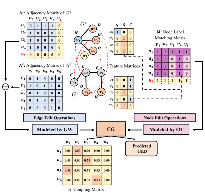
The load-bearing object is the coupling matrix produced by optimal transport. GEDIOT builds a cost matrix $\hat{C} = \tanh(H_1 W H_2^\top)$ from GNN embeddings, appends a dummy zero row to convert the matching constraints $\pi 1_{n_2} = 1_{n_1}$, $\pi^\top 1_{n_1} \leq 1_{n_2}$ into a standard optimal transport problem, and solves the entropy-regularized problem with a learnable Sinkhorn layer whose regularization coefficient $\varepsilon$ is optimized during training. The inner problem gives a coupling matrix $\hat{\pi}$ and a GED score $w_1 = \langle \hat{C}, \hat{\pi}\rangle$, supplemented by a neural tensor network score $w_2$. GEDGW adds dummy nodes to equalize graph sizes and solves $\min_{\pi} \langle \pi, M\rangle + \frac{1}{2}\langle \pi, \mathcal{L}(A_1, A_2) \otimes \pi\rangle$ over couplings using conditional gradient, where $M$ encodes label mismatch and $\mathcal{L}(A_1, A_2)$ encodes edge-pair mismatch. GEDHOT runs both and keeps the better value and the better edit path.
What would settle it
Run GEDIOT and GEDHOT on graphs with 11 to 25 nodes whose exact GED is known from an exact solver or a time-limited exhaustive A* search, compare the reported mean absolute error and feasibility against the synthetic edit-count labels, and check whether the min-ensemble's feasibility stays near 100% or drops because it systematically under-estimates; if the gains vanish or feasibility falls, the synthetic-ground-truth assumption is the culprit.
Extended reading notes
Core claim
The paper's central claim is that node matching in GED is a global decision, so the coupling matrix should be the transport plan obtained from a pairwise cost matrix, not the raw pairwise scores themselves. GEDIOT therefore learns only a cost matrix from node embeddings and feeds it through a differentiable Sinkhorn solver whose output is supervised against ground-truth matchings and GED values; this is an inverse optimal transport formulation, and it enforces the matching constraints during training. GEDGW shows that a purely unsupervised objective combining optimal transport for node label mismatch and insertions with Gromov-Wasserstein discrepancy for edge mismatch can already approximate GED well. The ensemble GEDHOT takes the smaller GED and the shorter edit path produced by the two, and the experiments report that this combination outperforms the strongest previous learning-based method on value, ranking, path, and generalization metrics.
Load-bearing premise
The evaluation treats synthetic GED values—generated by applying a known random number of edit operations to create each graph pair—as the correct ground truth for graphs larger than ten nodes, so the reported gains rest on that proxy being faithful to the true minimum edit distance.
Editorial extensions
If this is right
- Any GNN-based GED model that already produces a pairwise cost matrix can be upgraded by inserting a Sinkhorn layer after it, since the paper's improvement comes from the coupling step rather than from new vertex features.
- Unsupervised GEDGW achieves accuracy competitive with trained networks on some benchmarks, so meaningful GED approximation does not require ground-truth edit paths for training.
- GEDHOT inherits both the global-context matching of GEDIOT and the combinatorial structure of GEDGW, and the paper reports that it wins on GED value, ranking, edit-path quality, and triangle-inequality preservation.
- Inference remains polynomial, at $O(n^2)$ for GEDIOT and $O(K n^3)$ for GEDGW and GEDHOT, so the accuracy gains are available on graphs where exact A* search times out.
Reading between the lines
- A directly testable extension is to insert the same learnable-Sinkhorn coupling into other graph-matching pipelines, such as subgraph matching or graph similarity search, where the matching decision is likewise global; the paper does not run those experiments, but its coupling mechanism is pipeline-agnostic.
- Because GEDHOT keeps the minimum of two estimators, it is biased toward lower GED values; on synthetic ground truth generated by counting edit operations, this downward bias could inflate apparent accuracy, so the ensemble should be re-validated against exact GED on mid-size graphs.
- The paper's learnable entropy coefficient $\varepsilon$ offers a template for other optimal-transport-based neural layers that currently require manual regularization tuning; testing it in non-graph domains would show whether the benefit is specific to GED or generic.
- The reported gains on graphs with more than 10 nodes rest on synthetic labels; separating the architectural contribution from the synthetic-label bias would require evaluating on graphs of 11 to 25 nodes whose exact GED is computable.
Editorial analysis
A structured set of objections, weighed in public.
Referee Report
Summary. The paper proposes three methods for approximate graph edit distance (GED) computation and graph edit path (GEP) generation: GEDIOT, a supervised network that learns a vertex-pair cost matrix and derives the vertex coupling matrix through a learnable Sinkhorn (entropy-regularized optimal transport) layer; GEDGW, an unsupervised method that formulates GED as a linear combination of optimal transport and Gromov-Wasserstein discrepancy; and GEDHOT, an ensemble that takes the better of GEDIOT and GEDGW. The central claim is that deriving the coupling matrix from the cost matrix via OT captures global context and substantially improves GED accuracy over existing learning-based methods, with reported MAE reductions of 20.5%–63.8% (GEDIOT) and 31.2%–72.3% (GEDHOT) relative to GEDGNN. Experiments cover AIDS, Linux, IMDB, and synthetic power-law graphs, with additional ablations and generalizability studies.
Significance. If the central claim were established, the paper would make a meaningful contribution: it introduces a clean architectural idea (IOT-based coupling derivation) and an unsupervised OT/GW formulation that is competitive with learned methods. The manuscript includes several strengths: the OT derivations and Sinkhorn/CG implementations are mathematically sound; the code is released; the work connects GED computation to inverse optimal transport in a way that is novel relative to prior neural GED models that directly fit a matching matrix. The paper also provides error bounds (Appendix B.2) and a detailed complexity analysis. However, the experimental evidence does not currently isolate the effect of the OT mechanism, and a substantial part of the evaluation rests on synthetic ground truth for graphs larger than 10 nodes. These gaps are load-bearing for the paper's main thesis and must be addressed before the claims can be accepted.
major comments (3)
- [§6.4, Table 6] The ablation study does not isolate the effect of the OT module. Every variant in Table 6 (w/ GCN, w/o MLP, w/o Cost, w/o learnable ε) retains the Sinkhorn/OT layer; the only comparison that removes OT is GEDGNN, which differs from GEDIOT in multiple architectural dimensions (separate cost and matching cross-matrix modules, a different embedding architecture, an NTN-based graph discrepancy term, and a different loss balance). Consequently, the reported MAE improvements over GEDGNN could stem from these other differences rather than from deriving the coupling via optimal transport. To support the central claim, the authors should add an ablation that replaces the Sinkhorn layer with a direct coupling-fitting module (e.g., a softmax or MLP operating on the same cost matrix) while keeping all other GEDIOT components fixed.
- [§6.1 and Appendix F.1] For graphs with more than 10 nodes, the ground truth is not exact GED but a synthetic value: graph pairs are generated by applying a random number Δ of edit operations, and Δ is used as the ground truth. This applies to all IMDB results in Tables 3–5, Figure 8, and the power-law experiments in Appendix G.4. Because GEDGW and GEDHOT optimize objectives that are closely related to the edit-generation process, the reported performance on these datasets may reflect alignment with the generator rather than with exact GED. The paper should either limit its central claims to datasets with exact ground truth (AIDS and Linux) or provide evidence that the synthetic ground truth is a reliable proxy for exact GED on large graphs, for example by computing exact GED on a subset of large graph pairs where feasible.
- [§6.4] No measure of variance or statistical significance is reported for any metric. The abstract and Section 6.4 use the word "significantly" to describe improvements, but all results are single-run MAE, accuracy, ρ, τ, and p@k values without standard deviations, confidence intervals, or significance tests. Since GEDIOT and GEDHOT are compared against multiple baselines on three datasets, the authors should report means and standard deviations over at least several random seeds, and ideally paired significance tests (e.g., Wilcoxon signed-rank) for the comparisons against GEDGNN.
minor comments (6)
- [§4.2] The text says "as Eq. (12) is parameter-free" immediately after describing ε as a learnable parameter; the intended meaning appears to be that the iterative updates are fixed operations given ε, but the wording is confusing and should be clarified.
- [Appendix B.2, Theorem B.1] Theorem B.1 proves existence of a cost matrix bC* such that the entropy-regularized OT solution equals the ground-truth coupling, but the construction in Eq. (19) is not in the parametric family used by GEDIOT (bC = tanh(H1 W H2^T)). As written, the theorem does not justify the expressiveness of the actual architecture; the authors should either extend the result to the parameterized family or explicitly state the limitation.
- [Appendix E.2] There is a typo in "Algortihm 2" in the first sentence of Appendix E.2.
- [§5.1, Eq. (16)] The handling of dummy nodes in the node label matching matrix M is implicit: dummy rows in M are treated as having label mismatch with every real node of the other graph, but this is not stated. A sentence making the dummy-node convention explicit would improve reproducibility.
- [§6.2 and Table 3] The paper does not state whether the baseline numbers (SimGNN, GEDGNN, Noah, TaGSim, Classic) are taken from the original papers or reproduced with the same code and splits. This information is important for assessing the fairness of the comparison and should be reported in Appendix F.
- [§6.5, Figure 8] The generalizability experiment on "Large Unseen Graphs" relies on synthetic ground truth for IMDB graphs larger than 10 nodes; a short reminder of this in the caption or main text would prevent readers from misinterpreting the results as exact-GED performance.
Circularity Check
Minor circularity in synthetic-benchmark evaluation of GEDGW; the core GEDIOT derivation is self-contained.
-
self definitional
[Section 6.1 / Appendix F.1 (synthetic ground truth) and Appendix G.4 (power-law evaluation)]
"for the remaining graphs with more than 10 nodes, we use the ground-truth generation technique in [1, 35] to generate 100 synthetic graphs for each graph. ... Δ is regarded as an approximation of the ground truth GED∗(G,G′). ... the GED relative error of our GEDGW and GEDHOT is nearly 0 while that of GEDGNN is always almost 2."
GEDGW's objective (Eq. 17) is min_π ⟨π,M⟩ + (1/2)⟨π,L(A1,A2)⊗π⟩, which counts the edit operations induced by a matching (with a binary/continuous relaxation). The synthetic benchmark defines the ground-truth GED as the number Δ of edit operations applied to generate G′ from G. On these synthetic pairs, GEDGW's predicted value and the label are the same quantity by construction (up to relaxation and non-cancellation), so the reported near-zero relative error is a benchmark artifact, not independent evidence for GEDGW's accuracy. This does not affect the GEDIOT derivation, whose loss uses external ground-truth couplings/GEDs and whose coupling matrix is a learned function of the cost matrix.
full rationale
The paper's central derivation is not circular. GEDIOT is a supervised network: a GNN produces embeddings, a bilinear layer produces a cost matrix, a Sinkhorn layer produces a coupling matrix, and the loss fits both the coupling and the GED value to external ground truth. No equation equates the prediction to an input by construction; the cost matrix is learned, not set to the ground-truth-derived cost of Theorem B.1. GEDGW is a direct optimization formulation of GED and is not a fitted predictor. There is no load-bearing self-citation chain: the IOT, Sinkhorn, and GW references are external and their use does not assume the paper's conclusions. The only circularity found is in the synthetic large-graph benchmarks: the ground-truth label Δ is the number of edit operations used to generate the pair, which is exactly the quantity GEDGW minimizes, so GEDGW's near-zero relative error on power-law graphs is forced by the evaluation design. This is a minor, localized issue and does not undermine the exact-ground-truth comparisons on AIDS and Linux.
Assumptions & free parameters
free parameters (5)
- Cost matrix interaction matrix W =
learned, 32x32
- Sinkhorn regularization coefficient epsilon =
initialized 0.05, then learned
- Loss balancing hyperparameter lambda =
0.8
- Number of Sinkhorn iterations =
5
- Neural network parameters (GIN, MLP, NTN weights and biases) =
learned
assumptions (4)
- domain assumption Binary node matching can be relaxed to a doubly stochastic matrix without invalidating the GED objective.
- standard math The Sinkhorn algorithm converges to the unique solution of the entropy-regularized OT problem.
- domain assumption GED equals the minimum over permutations of node label mismatch plus edge mismatch costs.
- domain assumption Synthetic ground truth generated by applying a random number of edit operations is a valid proxy for exact GED on graphs with more than 10 nodes.
invented entities (2)
-
Dummy supernode in GEDIOT
-
Dummy nodes in GEDGW
Cite this review
Pith. "Pith review of Computing Approximate Graph Edit Distance via Optimal Transport." pith.science (2026). https://pith.science/paper/GN4AKKBM
@misc{pith2026241218857,
  author       = {Pith},
  title        = {Pith review of: Computing Approximate Graph Edit Distance via Optimal Transport},
  year         = {2026},
  howpublished = {\url{https://pith.science/paper/GN4AKKBM}},
  note         = {Machine review of arXiv:2412.18857}
}
abstract
Given a graph pair $(G^1, G^2)$, graph edit distance (GED) is defined as the minimum number of edit operations converting $G^1$ to $G^2$. GED is a fundamental operation widely used in many applications, but its exact computation is NP-hard, so the approximation of GED has gained a lot of attention. Data-driven learning-based methods have been found to provide superior results compared to classical approximate algorithms, but they directly fit the coupling relationship between a pair of vertices from their vertex features. We argue that while pairwise vertex features can capture the coupling cost (discrepancy) of a pair of vertices, the vertex coupling matrix should be derived from the vertex-pair cost matrix through a more well-established method that is aware of the global context of the graph pair, such as optimal transport. In this paper, we propose an ensemble approach that integrates a supervised learning-based method and an unsupervised method, both based on optimal transport. Our learning method, GEDIOT, is based on inverse optimal transport that leverages a learnable Sinkhorn algorithm to generate the coupling matrix. Our unsupervised method, GEDGW, models GED computation as a linear combination of optimal transport and its variant, Gromov-Wasserstein discrepancy, for node and edge operations, respectively, which can be solved efficiently without needing the ground truth. Our ensemble method, GEDHOT, combines GEDIOT and GEDGW to further boost the performance. Extensive experiments demonstrate that our methods significantly outperform the existing methods in terms of the performance of GED computation, edit path generation, and model generalizability.
Figures


Figures from the paper (16 more)






Reference graph
Works this paper leans on
-
[1]
Jiyang Bai and Peixiang Zhao. 2021. TaGSim: Type-Aware Graph Similarity Learning and Computation. PVLDB 15, 2 (2021), 335–347
work page 2021
-
[2]
Yunsheng Bai, Hao Ding, Song Bian, Ting Chen, Yizhou Sun, and Wei Wang. 2019. SimGNN: A Neural Network Approach to Fast Graph Similarity Computation. In WSDM. 384–392
work page 2019
-
[3]
David B Blumenthal and Johann Gamper. 2020. On The Exact Computation of The Graph Edit Distance. Pattern Recognition Letters 134 (2020), 46–57
work page 2020
-
[4]
Stephen Boyd and Lieven Vandenberghe. 2004. Convex Optimization. Cambridge University Press
2004
-
[5]
Gábor Braun, Alejandro Carderera, Cyrille W Combettes, Hamed Hassani, Amin Karbasi, Aryan Mokhtari, and Sebastian Pokutta. 2022. Conditional Gradient Methods. arXiv preprint arXiv:2211.14103 (2022)
arXiv 2022
-
[6]
Horst Bunke and Gudrun Allermann. 1983. Inexact Graph Matching for Structural Pattern Recognition. Pattern Recognition Letters 1, 4 (1983), 245–253
work page 1983
-
[7]
Lijun Chang, Xing Feng, Xuemin Lin, Lu Qin, Wenjie Zhang, and Dian Ouyang
-
[8]
Lijun Chang, Xing Feng, Kai Yao, Lu Qin, and Wenjie Zhang. 2022. Accelerating Graph Similarity Search via Efficient GED Computation. IEEE Transactions on Knowledge and Data Engineering 35, 5 (2022), 4485–4498
work page 2022
Show all 79 references
-
[9]
Laetitia Chapel, Mokhtar Z Alaya, and Gilles Gasso. 2020. Partial Optimal Trans- port with Applications on Positive-unlabeled Learning. NeurIPS 33 (2020), 2903– 2913
2020
-
[10]
Chandra R Chegireddy and Horst W Hamacher. 1987. Algorithms for Finding 𝑘-Best Perfect Matchings. Discrete Applied Mathematics 18, 2 (1987), 155–165
1987
-
[11]
Wei-Ting Chiu, Pei Wang, and Patrick Shafto. 2022. Discrete Probabilistic Inverse Optimal Transport. In ICML. 3925–3946
2022
-
[12]
Nicolas Courty, Rémi Flamary, Devis Tuia, and Alain Rakotomamonjy. 2016. Optimal Transport for Domain Adaptation. TPAMI 39, 9 (2016), 1853–1865
2016
-
[13]
Marco Cuturi. 2013. Sinkhorn Distances: Lightspeed Computation of Optimal Transport. NeurIPS 26 (2013), 2292–2300
2013
-
[14]
Yihe Dong and Will Sawin. 2020. COPT: Coordinated Optimal Transport on Graphs. NeurIPS 33 (2020), 19327–19338
2020
-
[15]
Stefan Fankhauser, Kaspar Riesen, and Horst Bunke. 2011. Speeding up Graph Edit Distance Computation Through Fast Bipartite Matching. In International Workshop on Graph-Based Representations in Pattern Recognition . 102–111
2011
-
[16]
Suen, Volkmar Frinken, Kaspar Riesen, and Horst Bunke
Andreas Fischer, Ching Y. Suen, Volkmar Frinken, Kaspar Riesen, and Horst Bunke. 2013. A Fast Matching Algorithm for Graph-Based Handwriting Recogni- tion. In International Workshop on Graph-Based Representations in Pattern Recog- nition (Lecture Notes in Computer Science, Vol...
2013
-
[17]
Karam Gouda and Mona Arafa. 2015. An Improved Global Lower Bound for Graph Edit Similarity Search. Pattern Recognition Letters 58 (2015), 8–14
2015
-
[18]
Karam Gouda and Mosab Hassaan. 2016. CSI_GED: An Efficient Approach for Graph Edit Similarity Computation. In 2016 IEEE 32nd International Conference on Data Engineering (ICDE) . IEEE, 265–276
2016
-
[19]
Weihua Hu, Bowen Liu, Joseph Gomes, Marinka Zitnik, Percy Liang, Vijay Pande, and Jure Leskovec. 2019. Strategies for Pre-training Graph Neural Networks. arXiv preprint arXiv:1905.12265 (2019)
2019 arXiv
-
[20]
Derek Justice and Alfred Hero. 2006. A Binary Linear Programming Formulation of The Graph Edit Distance. TPAMI 28, 8 (2006), 1200–1214
2006
-
[21]
Jongik Kim. 2021. Boosting Graph Similarity Search through Pre-computation. In Proceedings of the 2021 International Conference on Management of Data . 951–963
2021
-
[22]
Jongik Kim, Dong-Hoon Choi, and Chen Li. 2019. Inves: Incremental Partitioning- Based Verification for Graph Similarity Search.. In EDBT. 229–240
2019
-
[23]
Soheil Kolouri, Se Rim Park, Matthew Thorpe, Dejan Slepcev, and Gustavo K Rohde. 2017. Optimal Mass Transport: Signal Processing and Machine-Learning Applications. IEEE Signal Processing Magazine 34, 4 (2017), 43–59
2017
-
[24]
Ling Li, Siqiang Luo, Yuhai Zhao, Caihua Shan, Zhengkui Wang, and Lu Qin
-
[25]
Ruilin Li, Xiaojing Ye, Haomin Zhou, and Hongyuan Zha. 2019. Learning to Match via Inverse Optimal Transport. Journal of Machine Learning Research 20, 80 (2019), 1–37
2019
-
[26]
Yongjiang Liang and Peixiang Zhao. 2017. Similarity Search in Graph Databases: A Multi-Layered Indexing Approach. In ICDE. 783–794
2017
-
[27]
Yongjiang Liang and Peixiang Zhao. 2017. Similarity Search in Graph Databases: A Multi-layered Indexing Approach. In 2017 IEEE 33rd International Conference on Data Engineering (ICDE) . IEEE, 783–794
2017
-
[28]
Junfeng Liu, Min Zhou, Shuai Ma, and Lujia Pan. 2023. MATA*: Combining Learn- able Node Matching with A* Algorithm for Approximate Graph Edit Distance Computation. In CIKM. 1503–1512
2023
-
[29]
Facundo Mémoli. 2011. Gromov-Wasserstein Distances and The Metric Approach to Object Matching. Foundations of Computational Mathematics 11, 4 (2011), 417– 487
2011
-
[30]
James Munkres. 1957. Algorithms for the Assignment and Transportation Prob- lems. Journal of the society for industrial and applied mathematics 5, 1 (1957), 32–38
1957
-
[31]
Michel Neuhaus, Kaspar Riesen, and Horst Bunke. 2006. Fast Suboptimal Algo- rithms for The Computation of Graph Edit Distance. In Joint IAPR International Workshops on Statistical Techniques in Pattern Recognition (SPR) and Structural and Syntactic Pattern Recognition (SSPR) . 163–172
2006
-
[32]
Hermina Petric Maretic, Mireille El Gheche, Giovanni Chierchia, and Pascal Frossard. 2019. GOT: An Optimal Transport Framework for Graph Comparison. NeurIPS 32 (2019), 13899–13910
2019
-
[33]
Gabriel Peyré, Marco Cuturi, et al. 2019. Computational Optimal Transport: With Applications to Data Science. Foundations and Trends® in Machine Learning 11, 5-6 (2019), 355–607
2019
-
[34]
Gabriel Peyré, Marco Cuturi, and Justin Solomon. 2016. Gromov-Wasserstein Averaging of Kernel and Distance Matrices. In ICML. 2664–2672
2016
-
[35]
Chengzhi Piao, Tingyang Xu, Xiangguo Sun, Yu Rong, Kangfei Zhao, and Hong Cheng. 2023. Computing Graph Edit Distance via Neural Graph Matching.PVLDB 16, 8 (2023), 1817–1829
2023
-
[36]
Shaima Qureshi et al. 2023. Limits of Depth: Over-Smoothing and Over-Squashing in GNNs. Big Data Mining and Analytics 7, 1 (2023), 205–216
2023
-
[37]
Rishabh Ranjan, Siddharth Grover, Sourav Medya, Venkatesan Chakaravarthy, Yogish Sabharwal, and Sayan Ranu. 2022. Greed: A Neural Framework for Learning Graph Distance Functions. In NeurIPS. 22518–22530
2022
-
[38]
Kaspar Riesen and Horst Bunke. 2008. IAM Graph Database Repository for Graph Based Pattern Recognition and Machine Learning. In Joint IAPR International Workshops on Statistical Techniques in Pattern Recognition (SPR) and Structural and Syntactic Pattern Recognition (SSPR) (Le...
2008
-
[39]
Kaspar Riesen and Horst Bunke. 2009. Approximate Graph Edit Distance Com- putation by Means of Bipartite Graph Matching. Image and Vision Computing 27, 7 (2009), 950–959
2009
-
[40]
Kaspar Riesen, Sandro Emmenegger, and Horst Bunke. 2013. A Novel Software Toolkit for Graph Edit Distance Computation. In International Workshop on GraphBased Representations in Pattern Recognition . 142–151
2013
-
[41]
T Konstantin Rusch, Michael M Bronstein, and Siddhartha Mishra. 2023. A Survey on Oversmoothing in Graph Neural Networks. arXiv preprint arXiv:2303.10993 (2023)
2023 arXiv
-
[42]
Nino Shervashidze, Pascal Schweitzer, Erik Jan Van Leeuwen, Kurt Mehlhorn, and Karsten M Borgwardt. 2011. Weisfeiler-Lehman Graph Kernels. Journal of Machine Learning Research 12, 9 (2011), 2539–2561
2011
-
[43]
Liangliang Shi, Jack Fan, and Junchi Yan. 2024. OT-CLIP: Understanding and Generalizing CLIP via Optimal Transport. In ICML. 1–22
2024
-
[44]
Liangliang Shi, Zhaoqi Shen, and Junchi Yan. 2024. Double-Bounded Optimal Transport for Advanced Clustering and Classification. In AAAI, Vol. 38. 14982– 14990
2024
-
[45]
Liangliang Shi, Gu Zhang, Haoyu Zhen, Jintao Fan, and Junchi Yan. 2023. Un- derstanding and Generalizing Contrastive Learning from The Inverse Optimal Transport Perspective. In ICML. 31408–31421. Computing Approximate Graph Edit Distance via Optimal Transport Conference acrony...
2023
-
[46]
Andrew M Stuart and Marie-Therese Wolfram. 2020. Inverse Optimal Transport. SIAM J. Appl. Math. 80, 1 (2020), 599–619
2020
-
[47]
Vayer Titouan, Nicolas Courty, Romain Tavenard, and Rémi Flamary. 2019. Opti- mal Transport for Structured Data with Application on Graphs. In ICML. 6275– 6284
2019
-
[48]
Titouan Vayer, Laetitia Chapel, Rémi Flamary, Romain Tavenard, and Nicolas Courty. 2020. Fused Gromov-Wasserstein Distance for Structured Objects. Algo- rithms 13, 9 (2020), 212
2020
-
[49]
Titouan Vayer, Nicolas Courty, Romain Tavenard, Laetitia Chapel, and Rémi Flamary. 2019. Optimal Transport for Structured Data with Application on Graphs. In ICML, Vol. 97. PMLR, 6275–6284
2019
-
[50]
Cédric Villani et al. [n. d.]. Optimal Transport: Old and New . Vol. 338. Springer
-
[51]
Cédric Vincent-Cuaz, Rémi Flamary, Marco Corneli, Titouan Vayer, and Nicolas Courty. 2021. Semi-Relaxed Gromov-Wasserstein Divergence and Applications on Graphs. In ICLR. 1–14
2021
-
[52]
Hanchen Wang, Rong Hu, Ying Zhang, Lu Qin, Wei Wang, and Wenjie Zhang
-
[53]
Jianwei Wang, Kai Wang, Xuemin Lin, Wenjie Zhang, and Ying Zhang. 2024. Neural Attributed Community Search at Billion Scale. PACMMOD 1, 4 (2024), 1–25
2024
-
[54]
Runzhong Wang, Tianqi Zhang, Tianshu Yu, Junchi Yan, and Xiaokang Yang
-
[55]
Xiaoli Wang, Xiaofeng Ding, Anthony K. H. Tung, Shanshan Ying, and Hai Jin
-
[56]
Alan Geoffrey Wilson. 1969. The Use of Entropy Maximising Models, in the Theory of Trip Distribution, Mode Split and Route Split. Journal of Transport Economics and Policy (1969), 108–126
1969
-
[57]
Bing Xiao, Xinbo Gao, Dacheng Tao, and Xuelong Li. 2008. HMM-Based Graph Edit Distance for Image Indexing. International Journal of Imaging Systems and Technology 18, 2-3 (2008), 209–218
2008
-
[58]
Shunxin Xiao, Shiping Wang, Yuanfei Dai, and Wenzhong Guo. 2022. Graph Neural Networks in Node Classification: Survey and Evaluation. Machine Vision and Applications 33, 1 (2022), 4–22
2022
-
[59]
Hongteng Xu, Dixin Luo, and Lawrence Carin. 2019. Scalable Gromov- Wasserstein Learning for Graph Partitioning and Matching. In NeurIPS. 3046– 3056
2019
-
[60]
Jingjing Xu, Hao Zhou, Chun Gan, Zaixiang Zheng, and Lei Li. 2021. Vocabulary Learning via Optimal Transport for Neural Machine Translation. In ACL. 1–13
2021
-
[61]
Keyulu Xu, Weihua Hu, Jure Leskovec, and Stefanie Jegelka. 2018. How Powerful Are Graph Neural Networks? arXiv preprint arXiv:1810.00826 (2018)
2018 arXiv
-
[62]
Lei Yang and Lei Zou. 2021. Noah: Neural-Optimized A* Search Algorithm for Graph Edit Distance Computation. In ICDE. 576–587
2021
-
[63]
Weijie Yu, Zhongxiang Sun, Jun Xu, Zhenhua Dong, Xu Chen, Hongteng Xu, and Ji-Rong Wen. 2022. Explainable Legal Case Matching via Inverse Optimal Transport-based Rationale Extraction. In SIGIR. 657–668
2022
-
[64]
Zhiping Zeng, Anthony KH Tung, Jianyong Wang, Jianhua Feng, and Lizhu Zhou
-
[65]
Muhan Zhang. 2022. Graph Neural Networks: Link Prediction. Graph Neural Networks: Foundations, Frontiers, and Applications (2022), 195–223
2022
-
[66]
Muhan Zhang and Yixin Chen. 2018. Link Prediction Based on Graph Neural Networks. NeurIPS 31 (2018), 5171–5181
2018
-
[67]
Wei Zhang, Zihao Wang, Jie Fan, Hao Wu, and Yong Zhang. 2024. Fast Gradient Computation for Gromov-Wasserstein Distance. Journal of Machine Learning 3, 3 (2024), 282–299
2024
-
[68]
Kangfei Zhao, Jeffrey Xu Yu, Hao Zhang, Qiyan Li, and Yu Rong. 2021. A Learned Sketch for Subgraph Counting. In SIGMOD. 2142–2155
2021
-
[69]
Xiang Zhao, Chuan Xiao, Xuemin Lin, Qing Liu, and Wenjie Zhang. 2013. A Partition-Based Approach to Structure Similarity Search. PVLDB 7, 3 (2013), 169–180
2013
-
[70]
Xiang Zhao, Chuan Xiao, Xuemin Lin, and Wei Wang. 2012. Efficient Graph Similarity Joins with Edit Distance Constraints. In ICDE. IEEE, 834–845
2012
-
[71]
Xiang Zhao, Chuan Xiao, Xuemin Lin, Wenjie Zhang, and Yang Wang. 2018. Efficient Structure Similarity Searches: A Partition-based Approach. The VLDB Journal 27, 1 (2018), 53–78
2018
-
[72]
Weiguo Zheng, Lei Zou, Xiang Lian, Dong Wang, and Dongyan Zhao. 2013. Graph Similarity Search with Edit Distance Constraint in Large Graph Databases. In CIKM. 1595–1600
2013
-
[73]
Jie Zhou, Ganqu Cui, Shengding Hu, Zhengyan Zhang, Cheng Yang, Zhiyuan Liu, Lifeng Wang, Changcheng Li, and Maosong Sun. 2020. Graph Neural Networks: A Review of Methods and Applications. AI Open 1 (2020), 57–81. Conference acronym ’XX, June 03–05, 2018, Woodstock, NY Qihao Ch...
2020
-
[2009]
PVLDB 2, 1 (2009), 25–36
Comparing Stars: On Approximating Graph Edit Distance. PVLDB 2, 1 (2009), 25–36
2009
-
[2012]
An Efficient Graph Indexing Method. In ICDE. 210–221
-
[2020]
Speeding up GED Verification for Graph Similarity Search. In ICDE. 793– 804
-
[2021]
Combinatorial Learning of Graph Edit Distance via Dynamic Embedding. In CVPR. 5241–5250
-
[2022]
In SIGMOD
Neural Subgraph Counting with Wasserstein Estimator. In SIGMOD. 160– 175
-
[2023]
COCLEP: Contrastive Learning-based Semi-Supervised Community Search. In ICDE. 2483–2495
Reviewed August 11, 2026 · model on record in the stance chip above.
Discussion (0). Continue with ORCID to comment.