Pith. sign in

REVIEW 3 major objections 5 minor 15 references

Cosmic Whispers of the Early Universe: Gravitational Waves and Dark Matter from Primordial Black Holes

T0 review · 3 major / 5 minor · reviewed 2026-08-10 · deepseek-v4-flash

Pith's one-line read Broadest profiles set the critical compaction threshold at 2/5

desk verdict A systematic compilation of PBH abundance methods; the 'always 2/5' threshold for broad spectra is an extrapolation that needs testing, not a settled result. read the letter →

arxiv 2501.03065 v1 pith:RAXSKJSE submitted 2025-01-06 astro-ph.CO gr-qchep-ph

classification astro-ph.COgr-qchep-ph
keywords PrimordialblackholesCriticalcollapseCompactionfunctionThresholdstatisticsBroadpowerspectrumNon-GaussianitiesGravitationalwavesDarkmatter
topics Dark Matter
verification ladder T0 review T1 audit T2 compute T3 formal

The pith

A machine-rendered reading of the paper's core claim, the machinery that carries it, and where it could break.

The reading

This thesis tries to establish a sharper rule for when an overdensity in the early universe collapses into a primordial black hole. It argues that, for the broad and non-peaked power spectra that realistic inflationary models tend to produce, the critical threshold is set not by the statistically average compaction profile but by the broadest profiles. The threshold then takes a universal value, 2/5, independent of the shape of the power spectrum. If this is right, standard abundance computations that use average profiles need revision, and the change matters for how much dark matter PBHs can explain and for the gravitational-wave backgrounds associated with their formation.

What carries the argument

The load-bearing object is the compaction function $C(r)$, twice the local mass excess over the areal radius, which on superhorizon scales reads $C(r)=-2\Phi r\,\zeta'(r)[1+\tfrac{r}{2}\zeta'(r)]$. Collapse occurs when its maximum exceeds a threshold $C_{\rm th}$ that depends on the peak curvature $q=-\tfrac{r_m^2 C''(r_m)}{4C(r_m)}$, with $C_{\rm th}(q)$ running from $2/3$ for spiky profiles to $2/5$ for broad ones. The abundance calculation is carried by the joint Gaussian probability of the compaction and the curvature perturbation, with a correlation parameter $\gamma$ that is near unity for peaked spectra and small for broad spectra. Minimizing the effective squared threshold in $q$ pushes the dominant contribution to $q=0$ once $\gamma$ falls below a critical value, which is the mechanism that makes $2/5$ universal. The volume-averaged compaction, $\bar{C}(R_m)=\frac{3}{R_m^3}\int_0^{R_m} dx\,x^2 C(x)$, has threshold $2/5$ for both spiky and broad profiles, providing the profile-independent extension.

What would settle it

Numerical relativity simulations of collapse starting from a set of broad, non-peaked initial profiles with the same compaction maximum but different peak curvatures should find the critical compaction threshold equal to $2/5$ in every case; a spread in thresholds, or values clearly different from $2/5$, would falsify the universal-threshold claim.

Watch

Extended reading notes

Core claim

The paper's central claim is that the relevant critical threshold for primordial black hole formation from critical collapse is the one corresponding to the broadest compaction profiles whenever the curvature power spectrum is not sharply peaked. Concretely, the threshold function $C_{\rm th}(q)$, which grows from $2/5$ to $2/3$ as the curvature at the compaction peak increases, enters the abundance integral through an effective threshold; for broad spectra, parametrized by a small correlation parameter $\gamma$, the effective threshold is minimized at $q=0$, forcing $C_{\rm th}=2/5$. The same conclusion holds in the non-Gaussian case for the logarithmic USR-type relation. For very peaked spectra, by contrast, the average profile remains the right choice. The thesis also shows that the volume average of the compaction function has a profile-independent threshold of $2/5$, a step toward an observable with no shape dependence.

Load-bearing premise

The universal $2/5$ threshold holds if the numerically fitted threshold function $C_{\rm th}(q)$ is accurate for every profile shape and if the minimum of the effective threshold really sits at $q=0$ for broad, non-Gaussian spectra; if either fails, the universal value does not follow.

Editorial extensions

If this is right

  • For any non-peaked power spectrum, PBH abundance should be computed with the $2/5$ threshold rather than the average-profile threshold; this typically lowers the predicted abundance at a fixed amplitude.
  • Peaked spectra remain governed by the average profile, so the universal threshold applies only once the spectrum is sufficiently broad.
  • The result extends to the non-Gaussian case for positive, log-type non-Gaussianity, so the $2/5$ rule survives beyond Gaussian statistics.
  • Because thresholds enter abundances exponentially, small threshold changes translate into large abundance changes, and retuning the power-spectrum amplitude to compensate changes other predictions such as the induced gravitational-wave signal.
  • A profile-independent observable, the volume average of the compaction, can be used with threshold $2/5$; its statistics reduce to computing connected cumulants of the volume-averaged compaction.

Reading between the lines

Editorial extensions of the paper, not claims the author makes directly.

  • If the $2/5$ threshold is universal for broad spectra, published PBH constraints that were derived with average-profile thresholds may need to be re-derived; the direction and size of the shift will depend on each model's spectrum width.
  • The volume-averaged compaction route suggests a practical test: compute the one-point statistics of $\bar C(R_m)$ directly from the curvature power spectrum and compare PBH abundances against threshold-statistics results; numerical simulations can then settle whether $2/5$ is truly independent of profile.
  • Because the broadest profiles are rare, the claim implies that PBH formation selects atypical fluctuations; if confirmed, this would also affect predictions for the clustering and spin distribution of PBHs, since the collapsing profiles are not the average ones.
Share X Bluesky LinkedIn Reddit HN

Editorial analysis

A structured set of objections, weighed in public.

Desk editor's note, referee report, and a circularity audit.

Referee Report

3 major / 5 minor

Summary. This PhD thesis develops a comprehensive framework for computing the primordial black hole (PBH) abundance from inflationary curvature perturbations, with emphasis on primordial non-Gaussianities, threshold statistics on the compaction function, and the dependence of the collapse threshold on the compaction profile. It derives a master formula for the abundance with arbitrary local non-Gaussianity (Eq. 3.58), generalizes it to the PBH mass function (Eq. 3.68), and proposes in Sec. 3.3 that for non-peaked power spectra the abundance is dominated by the broadest compaction profiles, with a claimed universal threshold C_th = 2/5. The thesis then applies these tools to update LVK O3 and PTA constraints, discusses scalar-induced gravitational waves, and analyzes single-field ultra slow-roll and curvaton production models. The abstract and conclusions present PBHs as potential dark matter candidates and as a possible source of the PTA signal.

Significance. If the 'always 2/5' claim survives scrutiny, it is an important result: abundance predictions for broad power spectra would shift by orders of magnitude relative to average-profile prescriptions, with direct consequences for PBH-dark-matter and PTA interpretations. The manuscript is strong in presenting exact resummation-based formulas, in carefully assessing the convergence of perturbative expansions, and in spelling out applied constraints from LVK and PTA data. It also gives credit to the underlying numerical relativity inputs. However, the universal-threshold claim rests on an empirical fit to C_th(q) that has not been validated for the non-Gaussian profiles used in Sec. 3.3.3, and several phenomenological 'predictions' are obtained only after tuning the amplitude A to a target abundance. The core idea is promising, but at present the evidence is not yet at the level required for the strongest version of the claim.

major comments (3)
  1. [Sec. 3.2.2, Eq. (3.58); Sec. 3.2.3, Eq. (3.68)] The central claim that the threshold is 'always 2/5' for non-peaked power spectra is an extrapolation beyond the calibrated domain of Eq. (3.43). The numerical fit C_th(q) was calibrated on a restricted family of compaction profiles in Refs. [263,265]; the non-Gaussian map ζ = F(ζ_G) changes the relation between C_G, q, and C (Eqs. 3.49 and 3.104), so a profile with q → 0 in the non-Gaussian field is not guaranteed to have the same threshold as the q → 0 profile used to extract 2/5. The manuscript itself notes in Sec. 3.2.1 (footnote 6) that primordial non-Gaussianity can shift δ_c by a few percent for |f_NL| < O(5), yet Sec. 3.3.3 keeps C_th(q) unchanged while using strongly non-Gaussian examples (µ* = 5/2, r_dec = 0.1). Because β depends exponentially on the threshold, even a 10% shift in C_th changes the amplitude A required for a fixed abundance by O(1) and propagates into all derived abundance and constraint results. A dedicated numerical relativity check of the dominant non-Gaussian profiles, or a clearly stated restriction of the universal claim to Gaussian curvature perturbations, is needed before the 'always 2/5' statement can be accepted.
  2. [Sec. 3.2.2, Eq. (3.58); Sec. 3.2.3, Eq. (3.68)] Several phenomenological conclusions are obtained by fixing the amplitude A to match a reference abundance (e.g., β ≃ 10^-16 in Fig. 3.8, or f_PBH = 1 in Fig. 3.11) and then interpreting the resulting mass function as a prediction. This is a consistency constraint rather than a parameter-free prediction: because β depends exponentially on A and C_th, a different threshold choice is reabsorbed by an O(1) change in A, as the thesis itself acknowledges around Figs. 3.5 and 3.8. The text should state more explicitly in each application which results are robust to this tuning and which are only illustrative; otherwise the distinction between 'prediction' and 'fit' is blurred in the abstract and in Chapter 5.
  3. [Sec. 3.2.1, Eq. (3.45); Sec. 3.3.4, Fig. 3.17] The manuscript uses two different thresholds for the same broad-power-spectrum case: C_th = 0.56 from the average-profile prescription (Eq. 3.45) and C_th = 2/5 from the broad-profile prescription (Section 3.3). The comparison in Fig. 3.17 is performed for a log-normal spectrum with Δ = 1 and fixed q = 0.5 and shows a ratio β/β_0 of order one, but this is a single benchmark. Because the abundance is exponentially sensitive to the threshold, a systematic scan in Δ, µ* (or r_dec), and q is needed to establish that the two prescriptions agree within the stated accuracy, or to justify replacing the 0.56 threshold by 2/5.
minor comments (5)
  1. [Sec. 3.2.2] The figure references 'fig.2.10' should read 'fig.3.10' in the three places where they appear in the text.
  2. [Sec. 4.1] The heading 'Classification of the costraints' contains a typo; it should be 'constraints'.
  3. [Eq. (3.43)] The formula for C_th(q) is typeset in a way that is ambiguous: the incomplete gamma function should be written with explicit parentheses, e.g., Γ(5/(2q)) − Γ(5/(2q), 1/q), to avoid confusion.
  4. [Throughout, especially Eqs. (3.27), (3.30), (3.78)] The symbol γ is overloaded: γ_m in Eq. (3.27), the critical-collapse exponent γ in Eq. (3.30), and the correlation coefficient γ in Eq. (3.78). Distinct symbols or a short nomenclature table would improve readability.
  5. [General structure] The thesis interleaves textbook review material with original computations, and it would benefit from an explicit statement in each chapter separating the author's own results from previously published work with which the thesis is in dialogue.

Circularity Check

0 steps flagged · score 0.0 of 10

No circularity found: the central 2/5 claim is a derived profile-selection rule applied to an externally calibrated threshold function, and the tuned amplitudes are benchmark normalizations rather than hidden predictions.

full rationale

The derivation chain in Chapter 3 is not circular. Section 3.2 introduces threshold statistics on the compaction function with the master formula (Eq. 3.58), and Section 3.3 derives, for broad power spectra, that the PBH abundance is dominated by the smallest-curvature (broadest) compaction profiles; this is done analytically for Gaussian fields (Eqs. 3.90-3.94) and numerically for a non-Gaussian ultra-slow-roll example (Fig. 3.16). The value 2/5 is then taken from the independent numerical-relativity fit C_th(q) in Eq. (3.43), whose small-q limit is given as C_th(q << 1) ≈ 2/5. The statement 'always 2/5' is thus a combination of a derived profile-selection rule and an externally calibrated threshold value, not an identity between output and input. The tuning of the amplitude A to beta ≈ 10^-16 or f_PBH = 1 in Figs. 3.8 and 3.11 is a normalization convention for benchmark models, not a claim that the normalization itself was predicted. The thesis explicitly acknowledges in footnote 6 that primordial non-Gaussianities may shift delta_c by a few percent while keeping C_th(q) unchanged; that is an extrapolation beyond the calibrated domain and a correctness risk, but not a circular reduction because the threshold function is not defined in terms of the abundance being computed. Self-citations are numerous (refs. [1], [6], [7], [8]), but the load-bearing numerical thresholds and the LVK/PTA data are external, and the thesis reproduces the derivations rather than merely citing them. No step of the claimed derivation chain reduces by construction to its own inputs.

Assumptions & free parameters 5 free parameters · 5 assumptions · 0 invented entities

No new particles or forces are introduced. The thesis relies on standard cosmology and the compaction-function collapse criterion, with several parameters fitted to simulations or tuned to match target abundances.

free parameters (5)
  • Amplitude A of curvature power spectrum = e.g., 9.2e-3 for broad spectrum (Sec 3.2.2)
    A is tuned so that β_NG ~ 10^-16 at a reference mass, used throughout to set PBH abundance.
  • Threshold C_th = 0.56 for broad spectra (Sec 3.2); 2/5 in Sec 3.3
    The critical threshold for compaction is taken from numerical simulations (refs [254,263,265]) rather than derived.
  • Critical collapse constants K and gamma = K ~ 3.3 (log-normal) or 4.36 (broad), gamma ~ 0.36
    Taken from numerical simulations of critical collapse (refs [75,256,257]).
  • r_dec (curvaton decay fraction) = varied in [0.1, 1] in benchmarks
    Model parameter controlling the amount of non-Gaussianity; not fitted to data but freely varied.
  • mu_star (USR parameter) = taken as free (e.g., 5/2 in Sec 3.3.3)
    Sets the amount of non-Gaussianity in the USR model; not derived in the thesis.
assumptions (5)
  • domain assumption PBH formation occurs when the compaction function exceeds a threshold C_th (Sec 3.2.1).
    This is the collapse criterion taken from refs [263,264] and used in all abundance computations.
  • domain assumption The curvature perturbation is a local function of a single Gaussian field, ζ = F(ζ_G) (Eq 3.2).
    Assumed for USR and curvaton models; if non-local, the derived PDFs and formulas do not apply.
  • domain assumption The threshold statistics (Press-Schechter-like) approach is valid for computing PBH abundance (Eq 3.30).
    The master formula integrates the joint PDF above threshold, ignoring spatial correlations beyond the smoothing scale.
  • domain assumption Benchmark power spectra (log-normal, broad) are representative (Eqs 3.25, 3.26).
    The results are derived for these specific shapes; conclusions may not hold for other spectra.
  • standard math Gaussianity of the underlying field ζ_G and conservation of probability (Eqs 3.15, 3.50).
    Used to derive the joint PDFs and to change variables.

how reviews work

0 comments
Cite this review

Pith. "Pith review of Cosmic Whispers of the Early Universe: Gravitational Waves and Dark Matter from Primordial Black Holes." pith.science (2026). https://pith.science/paper/RAXSKJSE

@misc{pith2026250103065,
  author       = {Pith},
  title        = {Pith review of: Cosmic Whispers of the Early Universe: Gravitational Waves and Dark Matter from Primordial Black Holes},
  year         = {2026},
  howpublished = {\url{https://pith.science/paper/RAXSKJSE}},
  note         = {Machine review of arXiv:2501.03065}
}
read the original abstract

Various mechanisms have been suggested for the formation of Primordial Black Holes (PBHs), and this thesis focuses on the standard mechanism based on the critical collapse of cosmological fluctuations. The underlying idea is that during inflation, a period of rapid expansion in the early Universe, large cosmological fluctuations could have been generated. After inflation, when the cosmic horizon reached a size comparable to these fluctuations, if the latter were high enough, they could collapse and form a PBH. Beyond the fascinating possibility that these compact objects might make up all or part of the Dark Matter (DM) we observe today, their formation and existence is also associated with the generation of gravitational waves (GWs). These waves could contribute to the merger events observed by the LIGO/Virgo/KAGRA Collaboration (LVK) or account for signals detected by pulsar timing array experiments (PTA). In the first part of this thesis, we investigate the PBH scenario, examining the computation of the abundance beyond the Gaussian paradigm. In the second part, we discuss how PBH formation can produce a stochastic GW background and how observations, related to recent experiments such as LVK and PTA collaborations, can help in distinguishing between different PBH production models. Finally, in the last part, we investigate some aspects of the interplay between black holes and fundamental physics in the early Universe, describing some characteristics and challenges of various PBH production models.

Figures

Figures reproduced from arXiv: 2501.03065 by the authors.

Figure 2.1
Figure 2.1. Top panel: Taken form ref.[159]. The left panel is the angular-separation–binned inter-pulsar correlations, measured from 2,211 distinct pairings with the 67-pulsar array using the frequentist optimal statistic, assuming maximum-a-posteriori pulsar noise parameters and γ = 13/4 common-process amplitude from a Bayesian inference analysis. The bin widths are chosen so that each includes approximately the same number o… view at source ↗
Figure 3.1
Figure 3.1. First few coefficients of the expansion in eq. (3.13) as function of rdec (both analytically and numerically). In the figures we plot each coefficient cn(rdec) rescaled by the appropriate power σ n−2 0 in order to give a more realistic comparison of their relative size. expansion in ζN seems an appropriate approximation, and that only the first few orders are enough to capture the full result (cf. fig. 3.1 with σ0 =… view at source ↗
Figure 3.2
Figure 3.2. Variances (right-side axis) and γm (left-side axis) computed according to, respectively, eq. (3.24) and eq. (3.27) in the case of the log-normal power spectrum (left panel , as function of σ) and the broad power spectrum (right panel , as function of kmax/kmin). As far as the variances are concerned, we show the cases with j = 0, 1, 2. As far as γm is concerned, the dotted red lines represent the analytic results gi… view at source ↗
Figures from the paper (65 more)
Figure 3.3
Figure 3.3. Figure 3.3: We fix rdec = 0.5. Left panel. On the left-side y-axis we plot the function ζ = log [X(rdec, ζG)] as function of the Gaussian field ζG (solid red line) and its power-series expansion ζ10 (dashed red line). The two lines are superimposed and indistinguishable only wit…
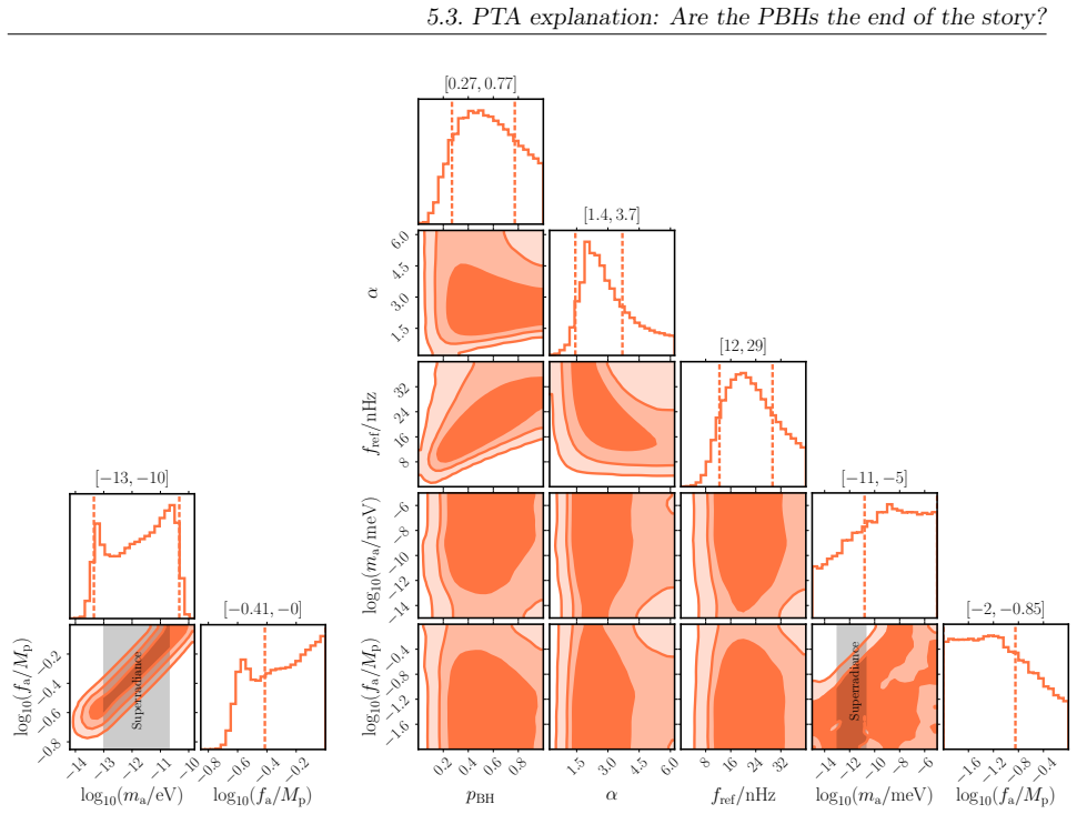
Figure 3.4
Figure 3.4. Figure 3.4: Computation of the primordial mass fraction β of the Universe stored into PBHs at the formation time done using the prescription in eq. (3.58). We consider the log-normal power spectrum in eq. (3.25) with fixed amplitude A and three different values of σ; from left t…
Figure 3.5
Figure 3.5. Figure 3.5: Left panel. Ratio βNL/βNG as function of the parameter rdec. We evaluate βNG at the quadratic order in the primordial NGs (see eq. (3.13) with N = 2) and considering the full resummed expression for ζ (see eq. (3.4)). We focus on the log-normal power spectrum in eq. …
Figure 3.6
Figure 3.6. Figure 3.6: We plot (left-side y axis, right panel) the relation k −1 = rm/κ in eq. (3.47) as function of rm. Both length scales k −1 and rm are written in units of k −1 min; from eq. (3.61), we read the corresponding horizon mass MH (rigth-side y axis). We set τ = rm and plot (…
Figure 3.7
Figure 3.7. Figure 3.7: Left (rdec = 0.5), central (rdec = 0.4) and right (rdec = 0.3) panels. We plot the NG mass fraction βNG computed according to eq. (3.58) and its expansion β (N) NG in as function of the expansion order N. We consider different choices for rmkmin, with τ = R ≡ rm in t…
Figure 3.8
Figure 3.8. Figure 3.8: Computation of βNG as a function of the horizon mass MH for different values of rdec. We fix kmin = 106 Mpc−1 and ∆k = 109 . The dashed black line corresponds to eq. (3.58) in which we only include the effect non-linearities (i.e. assuming the absence of primordial N…
Figure 3.9
Figure 3.9. Figure 3.9: Left panel. Variances σc,cr,r in eqs. (3.52-3.54) as function of the horizon mass MH. We take the parameters kmin = 106 Mpc−1 and ∆k = 109 , and normalize to 1 the amplitude of the power spectrum (we remind that the variances σc,cr,r simply scale as √ A). We also plo…
Figure 3.10
Figure 3.10. Figure 3.10: Top row. Contour lines indicate values of the probability density PG (CG, ζG). From the inner circle to the last purple one we locate values equally spaced in log scale in between 10−5 and 10−40 . The region between the red solid lines is the parameter space defined…
Figure 3.11
Figure 3.11. Figure 3.11: Mass function resulting from a broad power spectrum (solid lines, with kmin = 106 Mpc−1 and ∆k = 108.5 Mpc−1 ) and from a Log-Normal power spectrum (dashed lines, with σ = 0.5 and kpeak = 6×10¹² Mpc−1 ) with different amount of NGs, i.e. values of rdec. The amplitud…
Figure 3.12
Figure 3.12. Figure 3.12: Left panel. Height of the peak at the QCD Mass scale fSolar, assuming a broad power spectrum with kmin = 105 Mpc−1 as a function of the location of the asteroidal mass peak dominating the contribution to the dark matter. We compare the result obtained considering on…
Figure 3.13
Figure 3.13. Figure 3.13: Plot of qG min as a function of γ for σ2/σ0 = 2. 1.0 1.5 2.0 2.5 3.0 3.5 0.35 0.40 0.45 0.50 0.55 0.60 σ2/σ0 γcrit [PITH_FULL_IMAGE:figures/full_fig_p060_3_13.png]
Figure 3.15
Figure 3.15. Figure 3.15: The PBHs formation probability as a function of qG for σ0 = σ2/2 = 0.05 and three different values of γ = (0.3, 0.5, 0.8) for which ⟨qG⟩ = (0.6, 1, 1.6) for the Gaussian case. as long as CG(rm) < 4/3. The next step is to define the following Gaussian and correlated …
Figure 3.16
Figure 3.16. Figure 3.16: Mass fraction β for the non-Gaussian scenario computed with several values of ∆, where we fix µ∗ = 5/2, k∗rm = 2 and the amplitude of the power spectrum A = 10−2 . with µ⋆ a model-dependent parameter depending upon the transition between the ultra-slow-roll phase an…
Figure 3.17
Figure 3.17. Figure 3.17: Ratio between mass fraction β for the non-Gaussian case between the two prescriptions presented in this chapter. We fix the shape parameter q = 0.5 (as a consequence also the threshold using Eq. 3.43) and the shape of power spectrum ∆ = 1 while we vary the amplitude…
Figure 4.1
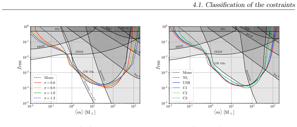
Figure 4.1. Figure 4.1: All constraints on the fraction of DM in the form of PBHs, fPBH, with mass MPBH, coming from PBH evaporation, microlensing, gravitational waves (LVK) and PBH accretion (CMB). Center [290] and gamma-ray observations by INTEGRAL [291, 292]. Similar constraints in this …
Figure 4.2
Figure 4.2. Figure 4.2: Examples of extended mass functions considered in this analysis. Left panel: Log-normal mass function with mc = 20M⊙. Right panel: Critical collapse mass function arising from a broken power￾law curvature power spectrum with α = 4, β = 0.5, different values of k∗, in…
Figure 4.3
Figure 4.3. Figure 4.3: Constraints for the monochromatic mass function detailing the contribution from R2 and R3 assuming that none of the observed events has a primordial origin. The constraints shown in gray are described in the main text and assume a monochromatic mass function. Results…
Figure 4.4
Figure 4.4. Figure 4.4: Same as Fig. (4.3), but for log-normal mass function (left panel) and critical collapse mass functions (right panel). Parameters for the latter are reported in [PITH_FULL_IMAGE:figures/full_fig_p080_4_4.png]
Figure 4.5
Figure 4.5. Figure 4.5: Posteriors for the BH binary merger rate model combining PBH and ABH binaries (blue) and for the model containing only ABH binaries (red). The PBH binaries are assumed to have a log-normal mass function with width σ = 0.6 and the ABH binaries are described by a pheno…
Figure 4.6
Figure 4.6. Figure 4.6: Constraints for a log-normal mass function with σ = 0.6 assuming that an arbitrary fraction of events can be primordial (solid red line) and that only astrophysical events have been observed (dashed red line). The constraints on the PBHs obtained from fitting the mix…
Figure 4.7
Figure 4.7. Figure 4.7: Left panel: Constraints from NANOGrav15 [159] on the amplitude of a log-normal curvature power spectrum, Eq. (3.25), with ∆ = 0.5 (blue), and on a broken power-law curvature power spectrum, Eq. (4.22), with α = 4, γ = 1 for β = 3 (pink) and β = 0.5 (red), assuming Ga…
Figure 4.8
Figure 4.8. Figure 4.8: Left panel: Constraints from NANOGrav15 [159] on the amplitude of a log-normal curvature power spectrum (3.25) with ∆ = 0.5 assuming Gaussian fluctuations and changing the window function. The horizontal lines correspond to fPBH = 1 using threshold statistics (solid)…
Figure 4.9
Figure 4.9. Figure 4.9: Left panels: Constraints from NANOGrav15 [159] on the amplitude of a log-normal curvature power spectrum (3.25) with ∆ = 0.5 (top panels) and on a broken power-law curvature power spectrum (4.22) with α = 4, γ = 1 for β = 3 (middle panels) and β = 0.5 (bottom panels)…
Figure 4.10
Figure 4.10. Figure 4.10: The NANOGrav15 constraints on the PBH abundance using threshold statistics assuming the two cases for the broken power law reported in Tab. 4.3 assuming the Gaussian approximation (solid) and with the full NG relation in Eq. (5.10). µ distortions and PBH seeds for S…
Figure 4.11
Figure 4.11. Figure 4.11: Constraints on the amplitude of the power spectrum, assuming negligible primordial NGs, from the FIRAS experiments, CMB, α-Lyman and NANOGrav15 for the same cases reported in Tab. 4.3. Consequently, the amplitude of the power spectrum in the range of scales related …
Figure 4.12
Figure 4.12. Figure 4.12: Left panel: Computation of the mass fraction β changing the NG parameters fNL and gNL with two benchmark cases for the log-normal power spectrum with an amplitude fixed to be A = 10−5 . Right panel: Computation of the PBH abundance fPBH changing the scale of the pea…
Figure 5.1
Figure 5.1. Figure 5.1: Spectral density of gravitational waves computed with rdec = 0.1 and rdec = 0.5 both with the broad spectrum (red lines) and with the log-normal spectrum (blue lines). The coloured dashed lines indicate instead the results when only contributions coming from non-line…
Figure 5.2
Figure 5.2. Figure 5.2: Top panel: Posterior for the parameters of a BPL model (4.22) for SIGWs, assuming no other source of GWs is present in both EPTA and NANOGrav15 data. The shaded regions in the off-diagonal panels show 2-D posteriors at the 1σ, 2σ, and 3σ confidence levels and the das…
Figure 5.3
Figure 5.3. Figure 5.3: PBH abundance for different NG models: non-linearities only (black), quasi-inflection-point models with β = 3 (red), curvaton models with rec = 0.9 (blue) and negative fNL (cyan). We assume a BPL power spectrum (4.22) with α = 4, β = 3 and γ = 1. The colored bands co…
Figure 5.4
Figure 5.4. Figure 5.4: The posterior probability distribution of the fit of the SMBH binary model with environmental effects to the NG15 data. The contours enclose the 1σ, 2σ, and 3σ CL regions. On top of each column, we report 1σ CL ranges. PTA data. This three-parameter model provides a …
Figure 5.5
Figure 5.5. Figure 5.5: The probability (5.18) for upward fluctuations in the SMBH model with environmental effects (green line) and the fluctuations measured in the NG15 data (orange line). 581]. Fluctuations in the GW spectrum As already mentioned, the SMBH signal may exhibit significant …
Figure 5.6
Figure 5.6. Figure 5.6: Contours of the minimal merger efficiency p min BH required for the probability of finding the candidate event at f ∼ 4nHz to exceed 5% for different values of the parameters of the environmental effects. In the black region, the probability of the candidate event is…
Figure 5.7
Figure 5.7. Figure 5.7: Left panel: The posterior probability distribution of the cosmic (super)string model fit to the NG15 data. The current (O3) LVK constraint and prospective future LVK sensitivity are shown by the solid and dashed lines. Right panel: Same as the left panel but includin…
Figure 5.8
Figure 5.8. Figure 5.8: Left panel: The posterior probability distribution of the phase transition fit to the NG15 data. The constraint from the production of PBHs is shown in grey. Right panel: Same as the left panel but including also SMBH binaries with environmental effects. 101 [PITH_F…
Figure 5.9
Figure 5.9. Figure 5.9: Left panel: The posterior probability distribution of the DW fit to the NG15 data. The dashed line indicates the ∆Neff bound, which constrains the possibility of DWs annihilating completely into dark radiation. Right panel: Same as the left panel but including also S…
Figure 5.10
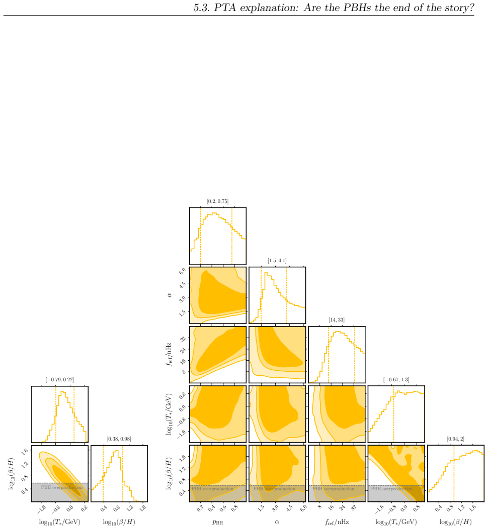
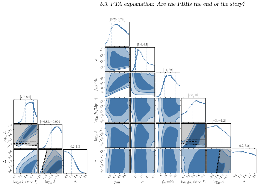
Figure 5.10. Figure 5.10: Left panel: The posterior probability distribution of the SIGW fit to the NG15 data. The black shaded region indicates where fPBH > 1, while the black dashed lines bracket the 1σ ranges in the marginalised direction.Right panel: Same as the left panel but including …
Figure 5.11
Figure 5.11. Figure 5.11: Left panel: The posterior probability distribution of the FOGW fit to the NG15 data. The black-shaded region shows the constraints by ∆Neff bound in Eq. (5.45), assuming fend = frh (solid line) and fend = 10frh (dashed line). We also show the r−nt correlation (5.46)…
Figure 5.12
Figure 5.12. Figure 5.12: Left panel: The posterior probability distribution of the “audible" axion fit to the NG15 data. The shaded region is excluded by super-radiance constraints. Right panel: Same as the left panel but including also SMBH binaries with environmental effects. from BBN (∆N…
Figure 5.13
Figure 5.13. Figure 5.13: Comparison of the best fits to the NG15 data for SMBH binaries with environmental effects and in the indicated BSM cosmological models. 5.3.3 Model comparisons [PITH_FULL_IMAGE:figures/full_fig_p120_5_13.png]
Figure 5.14
Figure 5.14. Figure 5.14: Extension of [PITH_FULL_IMAGE:figures/full_fig_p121_5_14.png]
Figure 6.1
Figure 6.1. Figure 6.1: Classical (top panel) and quantum (central panel) dynamics in the context of an explicit single-field model of inflation that exhibits the presence of a phase of USR in between the time interval Nin < N < Nend (cf. ref. [231]). In this specific realization, we have N…
Figure 6.2
Figure 6.2. Figure 6.2: Schematic evolution of η(N) in eq. (6.20) (top panel), ϵ(N) in eq. (6.23) (central panel) and dϵ2/dN (bottom panel) as function of the number of e-folds N. We explore different values of δN with the limit δN → 0 that corresponds to instantaneous transitions SR/USR at…
Figure 6.3
Figure 6.3. Figure 6.3: Left panel: Tree-level power spectrum using the reverse engineering approach. The numerical values of the other parameters are ηII = 3.5, ηIII = 0 and Nend − Nin = 2.5. In our parametrization, we go beyond the instantaneous transition approximation and we explore dif…
Figure 6.4
Figure 6.4. Figure 6.4: In both panels, we consider a generic USR dynamics with varying ηII (x-axis) and ∆NUSR (y-axis). We take ηIII = 0 and the instantaneous limit δN = 0. We plot in solid red contours of constant limδN→0 ∆P1−loop(k∗), defined in eq. (6.78) and computed according to eq. (…
Figure 6.5
Figure 6.5. Figure 6.5: Left panel: Graph of V ′′′/H as function of the background field value ϕ for two representative dynamics with, respectively, δN = 0.025 (dashed black) and δN = 0.4 (solid black). We compute the potential by means of the reverse engineering approach described in ref. …
Figure 6.6
Figure 6.6. Figure 6.6: Left panel: Comparison between the value of the full integral in eq. (6.100) and the analytical estimate in eq. (6.87). To mimic the instantaneous transition we take δN = 0.025. Right panel: We plot the ratio JδN (3, ∆NUSR) as function of δN. In both figures we take …
Figure 6.7
Figure 6.7. Figure 6.7: We consider a generic USR dynamics with varying ηII (x-axis) and ∆NUSR (y-axis). We take ηIII = 0 and the smooth limit δN = 0.4. The region hatched in red corresponds to ∆P1−loop(k∗) > 0. Along the line defined by the condition fPBH = 1, we get 100% of DM in the form…
Figure 6.8
Figure 6.8. Figure 6.8: Left: Value of ∆NUSR required in order to have fPBH = 1 for ηII = 3. Right: Different examples of evolution of η(N) responsible for the USR, assuming various δN and fixing ηII = 3. Dashed lines reports the scenario where δN is increased while ∆NUSR is kept fixed to t…
Figure 6.9
Figure 6.9. Figure 6.9: In both panels, we consider a USR dynamics with ηII = 3, ∆NUSR = 2.2, ηIII = 0 and the instantaneous limit δN = 0. These values corresponds to a scenario producing fPBH ≃ 1. The vertical gridlines corresponds to k = kin and kend in both panels. Left panel: correction…
Figure 6.10
Figure 6.10. Figure 6.10: Left: Expansion in time of the unperturbed Universe (time passes by along the y-axis); the Universe expands by the same amount at every point. Right: Expansion in time of the perturbed Universe. The long mode (ζL, blue) acts as a local rescaling of the scale factor,…
Figure 6.11
Figure 6.11. Figure 6.11: Left: Dynamics evolution (from right to the left) of the initial SR phase. The black dotted lines represent two benchmark solutions with large initial velocities, rapidly attracted by the SR trajectory (solid black line). Right: Dynamics evolution in presence of a U…
Figure 6.12
Figure 6.12. Figure 6.12: Illustrative schematic of the correction induced on the two-point correlator of long modes by a loop of short modes. On the right side, we plot the prototypical tree-level power spectrum of curvature perturbations as a function of the comoving wavenumber k in the pr…
Figure 6.13
Figure 6.13. Figure 6.13: Left panel: Power spectrum computed using the double inflection point potential with the parameters in tab. 6.4. In the pink panel it is the same power spectrum but zoomed on the relevant CMB scales. Central panel: Evolution of the horizon and the related mode k at …
Figure 6.14
Figure 6.14. Figure 6.14: Left panel: fPBH(MPBH) computed starting from the corresponding power spectrum in the Fig.6.13. Constraints on fPBH shown in the plot are addressed in sec. 4.Right panel: Evolution of the non￾gaussian parameter fNL computed using the Maldacena’s approximation (eq. 6…
Figure 6.15
Figure 6.15. Figure 6.15: Top panel: Values of the Hubble rate Hk when the related mode k crosses the horizon with different duration of the reheating ∆Nreh and wreh.The region shaded in gray corresponds to the condition log(k⋆/aeqHeq) < 1 computed according to eq. (6.128) assuming instantan…
Figure 7.1
Figure 7.1. Figure 7.1: Left panel: angular power spectrum for different choices of φ∗ and fH and fixed c = 27/16 (leading to a spectral growth nθ = 1.5). Right panel: different spectral growth as a function of ∆N depending on the assumed initial conditions for the radial field dynamics, i.…
Figure 7.2
Figure 7.2. Figure 7.2: The black line shows the evolution of the physical Hubble horizon 1/H as a function of the number of e-folds N, computed assuming slow-roll inflation and standard ΛCDM model. The green region shows the evolution of the scales associated with CMB observations. The sca…
Figure 7.3
Figure 7.3. Figure 7.3: Here we set f = 1015 GeV, Hinf/M¯ Pl = 10−6 , ϑ0 = 0.01. In the left panel we have mϕ = 5×10⁸ GeV, in the central panel mϕ = 108 GeV and in the right panel mϕ = 5×10⁷ GeV. The e-fold time difference ∆N between T = mϕ and H = Γϕ increases from left to right. This impl…
Figure 7.4
Figure 7.4. Figure 7.4: We fix f = 1015 GeV, Hinf/M¯ Pl = 10−6 , ϑ0 = 0.01. In the left panel, we show the evolution of r for the three values of mϕ shown in fig. 7.3; we also identify the value of rdec, defined as in eq. (7.35). In the right panel, we show the value of rdec as function of …
Figure 7.5
Figure 7.5. Figure 7.5: ϑ0 = 0.01. Scan over the parameter space of the model in light of the background analysis discussed in section 7.1.2. The horizontal dashed red line indicates the assumed re-heating temperature scale (7.13). The black hatched region identifies the parameter space for…
Figure 7.6
Figure 7.6. Figure 7.6: Same as in fig. 7.5 but for different values of ϑ0 (ϑ0 = 10−1 , dashed red lines; ϑ0 = 10−3 , dot-dashed blue lines; solid black lines refer to ϑ0 = 10−2 ). As far as Ndec is concerned, on the left panel we only show contours corresponding to Ndec = 15, 25, 35; simil…
Figure 7.7
Figure 7.7. Figure 7.7: Left panel. Power spectra Pζ (k) in eq. (7.38) for four different representative values of mϕ. We fix f = 3 × 10¹⁵ GeV and tune ϑ0 to get rdec = 0.5 in each of the four spectra. The dashed lines correspond to the sudden decay approximation while the solid lines inclu…
Figure 7.8
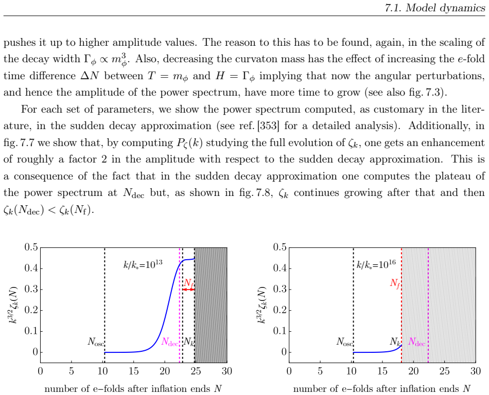
Figure 7.8. Figure 7.8: Growth of the curvature perturbation for different modes. Left panel: the mode k in exam re-enters the horizon at Nk > Ndec meaning that it still has some time to grow after the time of curvaton decay. This reflects in an enhancement in the amplitude of the power spe…
Figure 7.9
Figure 7.9. Figure 7.9: Left panel: broad power spectrum of the curvature perturbation obtained with the axion￾curvaton model assuming N∗ = 58. The black solid line refers to the power spectrum needed to obtain fPBH ≃ 1 when computing the abundance of PBHs with a non-perturbative treatment …
Figure 7.10
Figure 7.10. Figure 7.10: Signal of second order GWs associated with the broad power spectrum obtained within the curvaton model. When computing abundance of PBHs in the quadratic approximation (red line) and requir￾ing fPBH ≃ 1, one would find an amplitude which is smaller than the one requ…

Discussion (0). Continue with ORCID to comment.

Reference graph

Works this paper leans on

15 extracted references · 7 canonical work pages

  1. [1]

    IfthemodeiswayoutsidethehorizonatthebeginningoftheUSRphase, itstaysconstant even though its derivative exponentially grows because of the term∼ e−(3−2ηII)N

  2. [2]

    The curvature perturbation (and its derivative) grows because of the factor e−(3/2−ηII)N

    Consider a mode that crosses the Hubble horizon during the USR phase. The curvature perturbation (and its derivative) grows because of the factor e−(3/2−ηII)N. However, it is not immediate to find the exact scaling in time because in this case none of the approximations in eq.(C.4) can be applied. All the above features, even though obtained in the contex...

  3. [3]

    most fine-tuned

    + 3W−1(f∆N⋆)] ¯MPl , (C.17) where W−1(z) is the branch withk = −1 of the Lambert W functionWk(z). The scalar spectral index at the CMB pivot scale reads ns = 1 − 16 3[1 + W−1(f∆N⋆)]2 + 8 3[1 + W−1(f∆N⋆)] , (C.18) while for the tensor-to-scalar ratio we find r = 64 3[1 + W−1(f∆N⋆)]2 . (C.19) The amplitude of the scalar power spectrum at the CMB pivot scale...

  4. [744]

    Could MACHOS be primordial black holes formed during the QCD epoch? Phys

    Karsten Jedamzik. Could MACHOS be primordial black holes formed during the QCD epoch? Phys. Rept., 307:155–162, 1998. arXiv:astro-ph/9805147, doi:10.1016/S0370-1573(98) 00067-2

  5. [745]

    Simulations of PBH formation at the QCD epoch and comparison with the GWTC-3 catalog.JCAP, 05:004, 2023

    Albert Escrivà, Eleni Bagui, and Sebastien Clesse. Simulations of PBH formation at the QCD epoch and comparison with the GWTC-3 catalog.JCAP, 05:004, 2023. arXiv:2209.06196, doi:10.1088/1475-7516/2023/05/004

  6. [746]

    Gow, Christian T

    Andrew D. Gow, Christian T. Byrnes, Philippa S. Cole, and Sam Young. The power spectrum on small scales: Robust constraints and comparing PBH methodologies.JCAP, 02:002, 2021. arXiv:2008.03289, doi:10.1088/1475-7516/2021/02/002

  7. [747]

    Gravitational Waves Induced by Scalar Perturbations with a Lognor- mal Peak.JCAP, 09:037, 2020

    Shi Pi and Misao Sasaki. Gravitational Waves Induced by Scalar Perturbations with a Lognor- mal Peak.JCAP, 09:037, 2020. arXiv:2005.12306, doi:10.1088/1475-7516/2020/09/037

  8. [748]

    Log-dependent slope of scalar induced gravitational waves in the infrared regions.Phys

    Chen Yuan, Zu-Cheng Chen, and Qing-Guo Huang. Log-dependent slope of scalar induced gravitational waves in the infrared regions.Phys. Rev. D, 101(4):043019, 2020.arXiv:1910. 09099, doi:10.1103/PhysRevD.101.043019

Show all 15 references
  1. [749]

    Constraints on scalar-induced gravitational waves up to third order from a joint analysis of BBN, CMB, and PTA data.Phys

    Sai Wang, Zhi-Chao Zhao, and Qing-Hua Zhu. Constraints on scalar-induced gravitational waves up to third order from a joint analysis of BBN, CMB, and PTA data.Phys. Rev. Res., 6(1):013207, 2024. arXiv:2307.03095, doi:10.1103/PhysRevResearch.6.013207

  2. [750]

    Andrei D. Linde. Eternally existing selfreproducing inflationary universe.Phys. Scripta T, 15:169, 1987. doi:10.1088/0031-8949/1987/T15/024

  3. [751]

    A. S. Goncharov, Andrei D. Linde, and Viatcheslav F. Mukhanov. The Global Struc- ture of the Inflationary Universe. Int. J. Mod. Phys. A, 2:561–591, 1987. doi:10.1142/ S0217751X87000211

  4. [752]

    Largefieldpolynomialinflation: parameterspace, predictionsand (double) eternal nature.JCAP, 12:005, 2022.arXiv:2209.07545, doi:10.1088/1475-7516/ 2022/12/005

    ManuelDreesandYongXu. Largefieldpolynomialinflation: parameterspace, predictionsand (double) eternal nature.JCAP, 12:005, 2022.arXiv:2209.07545, doi:10.1088/1475-7516/ 2022/12/005

  5. [753]

    Gauging Fine-Tuning.Phys

    Feraz Azhar and Abraham Loeb. Gauging Fine-Tuning.Phys. Rev. D, 98(10):103018, 2018. arXiv:1809.06220, doi:10.1103/PhysRevD.98.103018

  6. [754]

    Axion isocurvature fluctuations with extremely blue spectrum

    Shinta Kasuya and Masahiro Kawasaki. Axion isocurvature fluctuations with extremely blue spectrum. Phys. Rev. D, 80:023516, 2009. arXiv:0904.3800, doi:10.1103/PhysRevD.80. 023516

  7. [755]

    Dark matter and the anthropic principle.Phys

    Simeon Hellerman and Johannes Walcher. Dark matter and the anthropic principle.Phys. Rev. D, 72:123520, 2005. arXiv:hep-th/0508161, doi:10.1103/PhysRevD.72.123520. 243 Appendix A Appendix of Chapter 3 A.1 On the convergence of the power-series expansion Consider the power seri...

Pith tools

Reviewed August 10, 2026 · model on record in the stance chip above.