REVIEW 2 major objections 5 minor 3 cited by
Phases of String Stars in the Presence of a Spatial Circle
T0 review · 2 major / 5 minor · reviewed 2026-08-10 · deepseek-v4-flash
Pith's one-line read String stars on a spatial circle change their phase structure with dimension; in d = 5 and d = 6, quartic corrections reverse the canonical and microcanonical stability ordering.
desk verdict New phase structure in d=2, 4, and 5 is real and mostly solid, but the d=6 canonical transition is not established because it rests on a branch the paper itself admits is outside the quartic EFT's validity. read the letter →
The pith
A machine-rendered reading of the paper's core claim, the machinery that carries it, and where it could break.
The reading
What carries the argument
The central object is the Horowitz-Polchinski effective field theory for the winding tachyon χ and radion φ near the Hagedorn temperature, truncated at quadratic order and then extended by quartic terms in the action (3.1). The quartic terms break the scaling invariance of the leading-order action, and it is precisely this breaking that resolves the d = 4 mass degeneracy and reverses the direction of temperature variation at d = 5. The numerical workhorse is the relaxation method on a compactified radial coordinate, seeded by localized higher-dimensional solutions, which generates entire non-uniform branches and their swallowtail phase diagrams.
What would settle it
Recompute the d = 6 phase diagram with |χ|^6 and other six-point terms included in the effective action; if the localized branch's free energy is no longer below the uniform branch near the critical point, or if the microcanonical stability reversal disappears, the paper's d = 6 conclusions fail.
Extended reading notes
Core claim
Working in Euclidean spacetime R^d × $S^{1}$_τ × $S^{1}$_z, the paper uses the Horowitz-Polchinski EFT—the action for the winding tachyon χ and the radion φ that encodes local variations of the Euclidean time circle—and its quartic-corrected extension to construct uniform and non-uniform string star solutions numerically. For 2 < d ≤ 4 the uniform string star gives way to non-uniform solutions through a second-order transition in the canonical ensemble, with the microcanonical ensemble showing a first-order swallowtail structure for 2 < d < 3; for d = 2 no such transition exists because a scaling symmetry of the uniform solution makes a critical point ambiguous. Including quartic terms changes the picture at d = 5: the non-uniform branch turns around, producing a first-order canonical transition with a swallowtail and a second-order microcanonical transition. Extending the same EFT to d = 6, the paper finds that near the critical point the canonical transition is first-order, while in the microcanonical ensemble string stars with small non-uniformity dominate even though they do not in the canonical ensemble; uniform string stars that are canonically stable become microcanonically unstable and vice versa. The paper also identifies a separate localized branch with lower free energy that would make the d = 6 transition first-order, while explicitly noting that this branch lies beyond the regime of validity of the EFT.
Load-bearing premise
The d = 5 and d = 6 conclusions assume the quartic-corrected action (3.1), with no |χ|^6 or higher couplings, is accurate in the regimes where free energies are compared; the paper itself notes this fails for the d = 6 localized branch, whose field amplitudes are not much smaller than one.
Editorial extensions
If this is right
- For 2 < d ≤ 4, the canonical transition from uniform to non-uniform string stars is second-order; the d = 4 mass degeneracy of the uniform branch is broken by quartic corrections, which make the mass increase with m∞.
- For d = 5, including quartic terms turns the canonical transition first-order with a swallowtail phase diagram and the microcanonical transition second-order, resolving the puzzle that the non-uniform phase always had higher free energy when quartic terms were neglected.
- For d = 6, near the critical point the canonical transition is first-order, while in the microcanonical ensemble small-nonuniformity solutions dominate and the uniform string star is anomalously stable when the spatial circle is larger than critical and unstable when it is smaller.
- For d = 2, there is no critical point connecting uniform and non-uniform solutions, because a scaling symmetry of the uniform solution makes any candidate critical length ambiguous; instead the Euclidean time circle opens up at infinity.
- For d = 3 and d = 4, the microcanonical ensemble does not transition from uniform to non-uniform string stars; at the critical mass the preferred endpoint is a localized black hole.
Reading between the lines
- If the d = 6 microcanonical reversal survives the inclusion of |χ|^6 terms, it would be a distinctive ensemble-dependent signature of string stars that has no analog in black-string Gregory-Laflamme physics; if the reversal disappears, the d = 6 phase diagram likely reduces to the d = 5 pattern.
- The d = 6 localized branch is computed outside the EFT's validity, so the paper's canonical first-order transition at d = 6 rests on an extrapolation; the same relaxation method applied to a fully resummed or stringy action would test whether the free-energy ordering persists.
- The d = 2 analysis suggests that in two spatial dimensions the very notion of a canonical ensemble for these solutions is ill-defined; a natural extension would be to interpret the uniform and non-uniform branches in terms of the parameter m∞ and check whether the scaling orbit of solutions has any physical observable.
- The same quartic-corrected EFT could be applied to string stars on tori with more than one compact circle, where non-uniformity in several directions could compete; the paper's d = 6 study was motivated by that question and shows the uniform branch may transition directly to a solution localized in all circle directions.
Editorial analysis
A structured set of objections, weighed in public.
Referee Report
Summary. This paper studies Euclidean string stars on R^d × S^1_τ × S^1_z using the Horowitz–Polchinski (HP) effective field theory, extended by the quartic terms of [48]. Section 2 analyzes the leading-order EFT: for d=2 the author finds non-uniform solutions with a logarithmically divergent radion and uniform solutions whose scaling symmetry (2.29) removes any critical point connecting the two branches; for 2<d<4 the numerical phase diagrams in the canonical and microcanonical ensembles reproduce and extend the results of [26, 27]. Section 3 adds the quartic-corrected action (3.1): the d=4 uniform-string mass degeneracy is resolved (the mass increases with m∞), the d=5 canonical phase diagram acquires a swallowtail with a first-order transition, and at d=6 the near-critical analysis yields an 'anomalous' microcanonical stability ordering opposite to the canonical one. The paper's headline claim for d=6 — that the uniform string star undergoes a first-order canonical transition into a localized string star — rests, however, on a branch that §3.3 concedes is 'already beyond the regime of validity' of the truncated action.
Significance. The paper's strongest parts are analytic and, for d≤5, well cross-checked. The d=2 scaling argument is a clean derivation of the absence of a uniform/non-uniform critical point in the marginal dimension, and the d=4 computation of Eqs. (3.4)–(3.6) determines the sign of the quartic mass shift without free parameters. The d=5 result, if numerically reliable, resolves a genuine puzzle left by [27], namely the absence of a lower-free-energy non-uniform branch at leading order, and the quoted ordering of transitions (canonical first-order, microcanonical second-order) is consistent with the independent perturbative analysis of [26]. The near-critical d=6 microcanonical instability (Fig. 11b) involves small-amplitude perturbations and is a sharp, falsifiable prediction. The analysis is not circular: phase diagrams are generated by solving the EFT (3.1), and [26] appears only as a perturbative cross-check. Against this, the d=6 canonical endpoint is not controlled beyond the EFT's validity, and the d=5 and d=6 numerical content is not accompanied by convergence tests or released code, so the quantitative phase-boundary locations have no stated accuracy.
major comments (2)
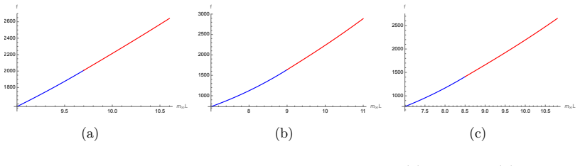
- [§3.3 (d=6), Figs. 12–13, Eq. (3.1)] The central d=6 claim that the uniform string star undergoes a first-order canonical transition into a localized string star is not established, because the branch that drives the transition is computed outside the regime of validity of the action (3.1). Section 3.3 concedes that this 'additional non-uniform branch' (Fig. 13) 'is already beyond the regime of validity,' and Fig. 13(b) shows χ(0,0) ≈ 0.465, i.e., an O(1) field. The quartic-truncated action omits |χ|^6, φ|χ|^4, and φ^3|χ|^2 interactions, whose relative weight at the core is O(χ^2) ≈ 0.2; these can shift the free energy of the localized branch by O(1) amounts and can even change whether the branch exists. The scaling argument offered in §3.3 (F_localized ≈ L-independent versus F_uniform ∝ L) controls only the parametric L→∞ limit; at the plotted L=180 the reported gap between the branches is only a factor ≈ 2 (F̃ ≈ 8.4×10^4 versus ≈ 4.5×10^4 in the units of Figs. 11(a) and 13(a)), and the comparison cannot be verified from the figures because of the normalization mismatch between Figs. 11(a) and 12(a). The statement that the localized branch extends all the way to m∞=0 also makes the phrase 'the uniform solution transitions at the critical point m∞≈0.00093' ambiguous, since the branch is presented as having lower free energy over the entire plotted range of m∞ rather than crossing the uniform branch at the critical point. The near-critical microcanonical results of Fig. 11(b) are not implicated, as they concern small-amplitude perturbations within the EFT's validity. To make the canonical claim load-bearing, the author should either estimate the leading omitted terms (or match onto the d≥7 construction of [29]) and show that the free-energy ordering is stable, or reframe the d=6 canonical transition — including the abstract's wording — as a conjecture supported by the scaling argument.
- [§2.2–§3.3, Figs. 5–13 (numerical method)] The quantitative phase diagrams for d=5 and d=6 (Figs. 10–13) are numerical solutions of the quartic-corrected EFT (3.1), but the paper reports no convergence tests, no residual tolerances, and no code or data release. The relaxation method on Lobatto–Chebyshev grids is described (citing [45]), yet the reader cannot assess whether the d=5 swallowtail turning point (m∞ ≈ 0.0097), the quoted d=5 critical value (m∞ ≈ 0.014 for L=200), the d=6 critical value (m∞ ≈ 0.00093 for L=180), or the existence of the 'additional non-uniform branch' of Fig. 13(a) are robust against grid resolution or continuation details. This is especially important where the d=6 branch is already outside the EFT's validity: without separating discretization error from EFT truncation error, the claimed phase-transition orders are not fully evidenced. Please add grid-resolution studies (e.g., doubling the u- and z-grid sizes), state the Newton/relaxation tolerances, and provide the code or a table of the plotted data.
minor comments (5)
- [§2.3, Eq. (2.29)] The scaling transformation in Eq. (2.29) is ambiguous as written: substituting χ̂ → λ²χ̂, φ̂ → λ²(φ̂+1)−1 together with r̂ → r̂/λ does not map solutions of (2.10) to solutions unless the coordinate rescaling is applied to the argument of the old profile; the consistent statement is (χ̃(r̂), φ̃(r̂)) = (λ²χ̂(λr̂), λ²(φ̂(λr̂)+1)−1), under which the periodicity m∞L is mapped to m∞L/λ, which is the property the subsequent argument uses. Please correct the formula so that the symmetry can be checked directly.
- [§3.3, Eq. (3.18)] The normalization instruction 'we can, for instance, set χ1(r) = 1' should specify a normalization at r = 0 (χ1(0) = 1); as written it is not a well-defined shooting condition for the linear system (3.18).
- [Figs. 11–13] The vertical scales of Figs. 11(a) and 12(a) are inconsistent for the same system (L = 180, κ/α′ = 1): near m∞ ≈ 0.00093 the rescaled free energy is plotted as F̃ ≈ 8.4 × 10^4 in Fig. 11(a) but as values of order 10^7 in Fig. 12(a). Because the central d=6 comparison is the ordering between the branch of Fig. 13(a) and the uniform branch, please state explicitly which normalization each figure uses, or replot them in common units.
- [§2.3, Fig. 6] For the microcanonical swallowtail diagrams of Fig. 6 (2 < d < 3), the text describes only the continuation from localized seeds with decreasing m∞L; a sentence explaining how the second non-uniform branch was obtained (analogous to the linear-combination seed of Eq. (3.16) at d=5) would make the construction reproducible.
- [§3.1, Fig. 9] The d=4 conclusion that the uniform mass increases with m∞ rests on the sign of the subleading fall-off coefficient Ĉ̂φ of Eq. (3.6), which is read off from a single numerical solution of (3.4) plotted in Fig. 9; reporting the numerical value of Ĉ̂φ (with a grid-convergence check) would make the claim quantitatively reproducible.
Circularity Check
No significant circularity: the phase diagrams are obtained by solving the EFT, with the quartic action taken from independent string-amplitude work and self-citations used only as cross-checks.
full rationale
The paper's central derivations are numerical solutions of the Horowitz-Polchinski EFT and its quartic-corrected extension (3.1). The quartic action is sourced from Ref. [48] (Brustein-Zigdon), an independent string-amplitude computation, not from the conclusions of this paper. The d=2, d=5, and d=6 phase structures are read off free-energy and entropy curves computed from the solved fields; no output quantity is fitted to impose the claimed transition order. Citations to the author's own [26] appear as consistency checks, such as 'consistent with the perturbative analysis in [26]' and 'as proposed in [26]' for a conjectured black-hole branch, but the phase diagrams themselves are generated by the shooting and relaxation numerics in the present work and by reproduction of the independent [27] results. The d=6 localized branch is admittedly 'already beyond the regime of validity' (Sec. 3.3), and the L-independence argument does not control omitted higher-order terms; this is a validity and correctness limitation, not a circular reduction, because the conclusion is not built into the equations being solved. No fitted parameter is renamed as a prediction, and no uniqueness theorem is imported from the author's own prior work. Overall the circularity burden is low.
Assumptions & free parameters
free parameters (1)
- κ/α' numerical normalization =
1
assumptions (6)
- domain assumption The HP EFT action (2.5) is the correct low-energy description of string stars near the Hagedorn temperature in R^d × S^1_z.
- domain assumption The quartic-corrected action (3.1), with only |χ|^4 and φ|χ|^2-type terms from [48], provides the next-to-leading correction for d=5 and d=6.
- domain assumption Spherical symmetry in x and reflection symmetry in z, with real χ, capture all relevant saddle points.
- standard math Canonical free energy and microcanonical entropy S = βM − βF determine phase dominance.
- domain assumption The Lobatto-Chebyshev relaxation and shooting solutions converge to the true continuum solutions.
- ad hoc to paper For d=2, the redefinition φhat = (1+r^2) φtilde with modified boundary conditions (2.28) selects the physical bounded solutions.
Cite this review
Pith. "Pith review of Phases of String Stars in the Presence of a Spatial Circle." pith.science (2026). https://pith.science/paper/RVPWYWSI
@misc{pith2026250103312,
  author       = {Pith},
  title        = {Pith review of: Phases of String Stars in the Presence of a Spatial Circle},
  year         = {2026},
  howpublished = {\url{https://pith.science/paper/RVPWYWSI}},
  note         = {Machine review of arXiv:2501.03312}
}
abstract
In string theory, black holes are expected to transition into string stars as their Hawking temperatures approach the Hagedorn temperature. We study string stars and their phase transitions in the Euclidean spacetime $\mathbb{R}^d\times\mathbb{S}_\tau^1\times\mathbb{S}_z^1$. Using the Horowitz-Polchinski (HP) effective field theory, we discover novel solutions for $d=2$. The uniform string star exhibits a scaling symmetry that results in the absence of a critical point for its transition into the non-uniform solution. For $d=4$, we show that quartic corrections to the effective action resolve the mass degeneracy of uniform string stars. At $d=5$, we find that as non-uniformity increases, the quartic terms become significant (while higher-order terms remain negligible) and reverse the direction of temperature variation, leading to a swallowtail-type phase diagram in the canonical ensemble. Extending the quartic-corrected EFT to $d=6$, we find that string stars with small non-uniformity dominate the microcanonical ensemble but not the canonical ensemble, similar to the $d=5$ case. However, in the microcanonical ensemble, the uniform string star is anomalously (un)stable when the spatial circle is larger (smaller) than the critical size.
Figures


Figures from the paper (10 more)



Forward citations
Cited by 3 Pith papers
-
Black Hole Entropy, Quantum Corrections and EFT Transitions
Quantum corrections to BPS black hole entropy in 4d N=2 string compactifications can be resummed into a finite formula that interpolates between four- and five-dimensional EFT descriptions and matches exact 5d microst...
-
IR Black Hole Instabilities Trigger Species-Scale Particle Production
A mechanism is proposed in which black hole instability at the tower scale converts a fraction of the mass into particles at the species scale, with Hawking evaporation subdominant.
-
A short overview on the Black Hole-Tower Correspondence and Species Thermodynamics
A review of the black hole-tower correspondence and species thermodynamics, which aim to explain black hole entropy via towers of light states and to show only certain towers are allowed.
Reference graph
Works this paper leans on
-
[27]
String theory in a pinch: resolving the Gregory-Laflamme singularity,
R. Emparan, M. Sanchez-Garitaonandia, and M. Tomašević, “String theory in a pinch: resolving the Gregory-Laflamme singularity,”JHEP 02 (2025) 104, arXiv:2411.14998 [hep-th]
arXiv 2025
-
[26]
From black strings to fundamental strings: non-uniformity and phase transitions,
J. Chu, “From black strings to fundamental strings: non-uniformity and phase transitions,” JHEP 04 (2025) 045, arXiv:2410.23597 [hep-th]
arXiv 2025
-
[48]
Effective field theory for closed strings near the Hagedorn temperature,
R. Brustein and Y. Zigdon, “Effective field theory for closed strings near the Hagedorn temperature,” JHEP 04 (2021) 107, arXiv:2101.07836 [hep-th]
arXiv 2021
- [29]
-
[45]
Numerical Methods for Finding Stationary Gravitational Solutions,
O. J. C. Dias, J. E. Santos, and B. Way, “Numerical Methods for Finding Stationary Gravitational Solutions,” Class. Quant. Grav. 33 no. 13, (2016) 133001, arXiv:1510.02804 [hep-th]
arXiv 2016
-
[1]
C. Callan, R. Myers, and M. Perry, “Black holes in string theory,”Nuclear Physics B 311 no. 3, (1989) 673–698. https://www.sciencedirect.com/science/article/pii/0550321389901727
arXiv 1989
-
[2]
Revisiting $R^4$ higher curvature corrections to black holes
Y. Chen, “Revisiting R4 higher curvature corrections to black holes,” arXiv:2107.01533 [hep-th]
-
[3]
Role of String Excitations in the Last Stages of Black Hole Evaporation,
M. J. Bowick, L. Smolin, and L. C. R. Wijewardhana, “Role of String Excitations in the Last Stages of Black Hole Evaporation,”Phys. Rev. Lett. 56 (1986) 424
work page 1986
Show all 51 references
-
[4]
Some speculations about black hole entropy in string theory,
L. Susskind, “Some speculations about black hole entropy in string theory,” arXiv:hep-th/9309145
-
[5]
A Correspondence principle for black holes and strings,
G. T. Horowitz and J. Polchinski, “A Correspondence principle for black holes and strings,” Phys. Rev. D 55 (1997) 6189–6197, arXiv:hep-th/9612146
1997 arXiv
-
[6]
Extremal black holes and elementary string states,
A. Sen, “Extremal black holes and elementary string states,”Mod. Phys. Lett. A 10 (1995) 2081–2094, arXiv:hep-th/9504147
1995 arXiv
-
[7]
Selfgravitating fundamental strings and black holes,
T. Damour and G. Veneziano, “Selfgravitating fundamental strings and black holes,” Nucl. Phys. B 568 (2000) 93–119, arXiv:hep-th/9907030
2000 arXiv
-
[8]
Selfgravitating strings and string / black hole correspondence,
R. R. Khuri, “Selfgravitating strings and string / black hole correspondence,”Phys. Lett. B 470 (1999) 73–76, arXiv:hep-th/9910122
1999 arXiv
-
[9]
Accelerating branes and the string/black hole transition,
D. Kutasov, “Accelerating branes and the string/black hole transition,” arXiv:hep-th/0509170
-
[10]
The Charged black hole/string transition,
A. Giveon and D. Kutasov, “The Charged black hole/string transition,”JHEP 01 (2006) 120, arXiv:hep-th/0510211
2006 arXiv
-
[11]
Fundamental strings and black holes,
A. Giveon and D. Kutasov, “Fundamental strings and black holes,”JHEP 01 (2007) 071, arXiv:hep-th/0611062
2007 arXiv
-
[12]
Selfgravitating fundamental strings,
G. T. Horowitz and J. Polchinski, “Selfgravitating fundamental strings,”Phys. Rev. D 57 (1998) 2557–2563, arXiv:hep-th/9707170
1998 arXiv
-
[13]
Black hole entropy sourced by string winding condensate,
R. Brustein and Y. Zigdon, “Black hole entropy sourced by string winding condensate,” JHEP 10 (2021) 219, arXiv:2107.09001 [hep-th]
2021 arXiv
-
[14]
String scale black holes at large D,
Y. Chen and J. Maldacena, “String scale black holes at large D,”JHEP 01 (2022) 095, arXiv:2106.02169 [hep-th]
2022 arXiv
-
[15]
On the black hole/string transition,
Y. Chen, J. Maldacena, and E. Witten, “On the black hole/string transition,”JHEP 01 (2023) 103, arXiv:2109.08563 [hep-th]
2023 arXiv
-
[16]
String stars in anti de Sitter space,
E. Y. Urbach, “String stars in anti de Sitter space,”JHEP 04 (2022) 072, arXiv:2202.06966 [hep-th]
2022 arXiv
-
[17]
Winding Tachyons and Stringy Black Holes,
B. Balthazar, J. Chu, and D. Kutasov, “Winding Tachyons and Stringy Black Holes,” arXiv:2204.00012 [hep-th] . – 24 –
-
[18]
On small black holes in string theory,
B. Balthazar, J. Chu, and D. Kutasov, “On small black holes in string theory,” JHEP 03 (2024) 116, arXiv:2210.12033 [hep-th]
2024 arXiv
-
[19]
High energy scattering and string/black hole transition,
A. Bedroya, “High energy scattering and string/black hole transition,” arXiv:2211.17162 [hep-th]
-
[20]
The black hole/string transition in AdS3 and confining backgrounds,
E. Y. Urbach, “The black hole/string transition in AdS3 and confining backgrounds,” JHEP 09 (2023) 156, arXiv:2303.09567 [hep-th]
2023 arXiv
-
[21]
The correspondence between rotating black holes and fundamental strings,
N. Čeplak, R. Emparan, A. Puhm, and M. Tomašević, “The correspondence between rotating black holes and fundamental strings,”JHEP 11 (2023) 226, arXiv:2307.03573 [hep-th]
2023 arXiv
-
[22]
Double winding condensate CFT,
I. Halder and D. L. Jafferis, “Double winding condensate CFT,”JHEP 05 (2024) 189, arXiv:2308.11702 [hep-th]
2024 arXiv
-
[23]
AdS3 String Stars at Pure NSNS Flux,
N. Agia and D. L. Jafferis, “AdS3 String Stars at Pure NSNS Flux,” arXiv:2311.04956 [hep-th]
-
[24]
The Tale of Three Scales: the Planck, the Species, and the Black Hole Scales,
A. Bedroya, C. Vafa, and D. H. Wu, “The Tale of Three Scales: the Planck, the Species, and the Black Hole Scales,”arXiv:2403.18005 [hep-th]
-
[25]
Self gravitating spinning string condensates,
J. E. Santos and Y. Zigdon, “Self gravitating spinning string condensates,”JHEP 07 (2024) 217, arXiv:2403.20332 [hep-th]
2024 arXiv
-
[28]
Size and Shape of Rotating Strings and the Correspondence to Black Holes,
N. Čeplak, R. Emparan, A. Puhm, and M. Tomašević, “Size and Shape of Rotating Strings and the Correspondence to Black Holes,”arXiv:2411.18690 [hep-th]
-
[30]
The dark dimension and the Swampland,
M. Montero, C. Vafa, and I. Valenzuela, “The dark dimension and the Swampland,” JHEP 02 (2023) 022, arXiv:2205.12293 [hep-th]
2023 arXiv
-
[31]
On nonuniform black branes,
S. S. Gubser, “On nonuniform black branes,”Class. Quant. Grav. 19 (2002) 4825–4844, arXiv:hep-th/0110193
2002 arXiv
-
[32]
Static axisymmetric vacuum solutions and nonuniform black strings,
T. Wiseman, “Static axisymmetric vacuum solutions and nonuniform black strings,” Class. Quant. Grav. 20 (2003) 1137–1176, arXiv:hep-th/0209051
2003 arXiv
-
[33]
Topology change in general relativity, and the black hole black string transition,
B. Kol, “Topology change in general relativity, and the black hole black string transition,” JHEP 10 (2005) 049, arXiv:hep-th/0206220
2005 arXiv
-
[34]
A Critical dimension in the black string phase transition,
E. Sorkin, “A Critical dimension in the black string phase transition,”Phys. Rev. Lett. 93 (2004) 031601, arXiv:hep-th/0402216
2004 arXiv
-
[35]
On black-brane instability in an arbitrary dimension,
B. Kol and E. Sorkin, “On black-brane instability in an arbitrary dimension,”Class. Quant. Grav. 21 (2004) 4793–4804, arXiv:gr-qc/0407058. – 25 –
2004 arXiv
-
[36]
On non-uniform smeared black branes,
H. Kudoh and U. Miyamoto, “On non-uniform smeared black branes,”Class. Quant. Grav. 22 (2005) 3853–3874, arXiv:hep-th/0506019
2005 arXiv
-
[37]
LG (Landau-Ginzburg) in GL (Gregory-Laflamme),
B. Kol and E. Sorkin, “LG (Landau-Ginzburg) in GL (Gregory-Laflamme),”Class. Quant. Grav. 23 (2006) 4563–4592, arXiv:hep-th/0604015
2006 arXiv
-
[38]
Instabilities of black strings and branes,
T. Harmark, V. Niarchos, and N. A. Obers, “Instabilities of black strings and branes,” Class. Quant. Grav. 24 (2007) R1–R90, arXiv:hep-th/0701022
2007 arXiv
-
[39]
High and Low Dimensions in The Black Hole Negative Mode,
V. Asnin, D. Gorbonos, S. Hadar, B. Kol, M. Levi, and U. Miyamoto, “High and Low Dimensions in The Black Hole Negative Mode,”Class. Quant. Grav. 24 (2007) 5527–5540, arXiv:0706.1555 [hep-th]
2007 arXiv
-
[40]
Evolution and End Point of the Black String Instability: Large D Solution,
R. Emparan, R. Suzuki, and K. Tanabe, “Evolution and End Point of the Black String Instability: Large D Solution,”Phys. Rev. Lett. 115 no. 9, (2015) 091102, arXiv:1506.06772 [hep-th]
2015 arXiv
-
[41]
Phases and Stability of Non-Uniform Black Strings,
R. Emparan, R. Luna, M. Martínez, R. Suzuki, and K. Tanabe, “Phases and Stability of Non-Uniform Black Strings,”JHEP 05 (2018) 104, arXiv:1802.08191 [hep-th]
2018 arXiv
-
[42]
Endpoint of the Gregory-Laflamme instability of black strings revisited,
P. Figueras, T. França, C. Gu, and T. Andrade, “Endpoint of the Gregory-Laflamme instability of black strings revisited,”Phys. Rev. D 107 no. 4, (2023) 044028, arXiv:2210.13501 [hep-th]
2023 arXiv
-
[43]
Black strings and p-branes are unstable,
R. Gregory and R. Laflamme, “Black strings and p-branes are unstable,”Phys. Rev. Lett. 70 (1993) 2837–2840, arXiv:hep-th/9301052
1993 arXiv
-
[44]
The Instability of charged black strings and p-branes,
R. Gregory and R. Laflamme, “The Instability of charged black strings and p-branes,” Nucl. Phys. B 428 (1994) 399–434, arXiv:hep-th/9404071
1994 arXiv
-
[46]
Black holes in a periodic universe,
A. R. Bogojevic and L. Perivolaropoulos, “Black holes in a periodic universe,”Mod. Phys. Lett. A 6 (1991) 369–376
1991
-
[47]
Black holes in a compactified space-time,
A. V. Frolov and V. P. Frolov, “Black holes in a compactified space-time,”Phys. Rev. D 67 (2003) 124025, arXiv:hep-th/0302085
2003 arXiv
-
[49]
Self-interacting fundamental strings and black holes,
D. Chialva, “Self-interacting fundamental strings and black holes,”Nucl. Phys. B 819 (2009) 256–281, arXiv:0903.3977 [hep-th]
2009 arXiv
-
[50]
Instant Folded Strings and Black Fivebranes,
A. Giveon, N. Itzhaki, and U. Peleg, “Instant Folded Strings and Black Fivebranes,” JHEP 08 (2020) 020, arXiv:2004.06143 [hep-th]
2020 arXiv
-
[51]
Stringy ER = EPR,
D. L. Jafferis and E. Schneider, “Stringy ER = EPR,”JHEP 10 (2022) 195, arXiv:2104.07233 [hep-th] . – 26 –
2022 arXiv
Reviewed August 10, 2026 · model on record in the stance chip above.
Discussion (0). Continue with ORCID to comment.