REVIEW 4 major objections 4 minor 1 cited by
Supervised Learning for Analog and RF Circuit Design: Benchmarks and Comparative Insights
T0 review · 4 major / 4 minor · reviewed 2026-08-10 · deepseek-v4-flash
Pith's one-line read This paper argues that supervised machine learning can invert the analog/RF design flow by predicting circuit parameters from performance specifications, with best mean relative errors of 0.30% on an LNA and 0.23% on a receiver.
desk verdict A solid, useful benchmark extension that is undermined by an unsupported headline number and by testing only on the same swept grid used to generate the data. read the letter →
The pith
A machine-rendered reading of the paper's core claim, the machinery that carries it, and where it could break.
The reading
What carries the argument
The load-bearing object is the supervised inverse map $M: \mathbb{R}^N \to \mathbb{R}^D$ that sends performance specifications to circuit parameters; for heterogeneous circuits the map is a composition of coupled sub-block maps $M_{\text{total}}(X) = f(M_1(x_1), M_2(x_2), M_3(x_3))$, which formalizes why higher dimensionality and block interactions demand more data. The map is trained with an $\ell^1$ loss on parameter values and evaluated through a two-stage pipeline: the model predicts $\hat{y}$, a circuit simulator computes the resulting performance $\hat{x}$, and the reported mean relative error compares $\hat{x}$ to the target $x$. This simulation-in-the-loop evaluation is what makes the accuracy figures meaningful for designers, because it measures end-to-end performance error rather than parameter-space distance.
What would settle it
Take a physically plausible performance target that lies outside the swept range of at least one circuit parameter, or on a combination not representable on the grid, run the trained model, simulate the predicted parameters, and measure the performance relative error; if errors rise sharply (for example, mean error above 10%) across models, the inverse-mapping claim is limited to grid interpolation rather than true design-space coverage.
Extended reading notes
Core claim
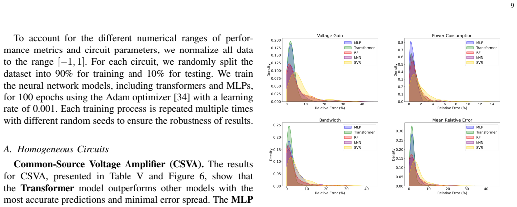
The paper establishes that the conventional analog/RF design loop can be reversed: given a desired performance specification vector $x$, a supervised model $y = M(x)$ predicts a set of circuit parameters, and the predicted parameters are then simulated to verify that the achieved performance matches the request. On the homogeneous benchmark, the low-noise amplifier is effectively solved (0.30% mean relative error with MLP, 100% of errors below 2%), whereas the power amplifier remains the hardest block (19.98% best mean error), showing that circuits with nonlinear trade-offs resist direct inversion. On heterogeneous systems, increasing the training set cuts error by 88%, and the receiver reaches 0.23% mean relative error with k-nearest neighbors, demonstrating that data scale, not model expressivity, is the dominant factor for these systems. The authors also report a model-complexity map: transformers and MLPs dominate on single-stage and cascode amplifiers, random forests on two-stage amplifiers and VCOs, MLP and kNN on the transmitter, and kNN on the receiver; support vector regression is consistently the weakest. The study is presented as a benchmark-oriented extension that turns a dataset into explicit guidelines for when each ML family is appropriate.
Load-bearing premise
The benchmark is generated by sweeping design parameters on a fixed grid and only evaluating on random points from that same grid, so the entire test is interpolation within the swept ranges and nothing is established about requests outside those ranges.
Editorial extensions
If this is right
- For circuits with near-linear parameter-performance relations, such as the LNA, the paper implies that manual sizing can be replaced by a single forward pass of a supervised model with sub-1% performance error.
- For complex blocks like the power amplifier, the best observed mean error of about 20% means ML-based sizing is not yet trustworthy for such circuits, and designers should still rely on optimization loops.
- For heterogeneous systems, the 88% error reduction from more training data shows that investing in simulation data, rather than switching models, is the most direct route to accuracy.
- The winning model family changes with circuit structure, so a practical workflow needs to select among MLP/transformer, random forest, and kNN based on circuit complexity and dataset size rather than assuming one method is best.
- The simulation-in-the-loop evaluation protocol should be a standard for future circuit-ML benchmarks, because parameter-space error alone does not tell a designer whether the target performance was met.
Reading between the lines
- Editorial: the reported accuracies are interpolation results on the swept grid; generalizing to arbitrary specification vectors outside the grid is unproven, so the headline 0.23% and 0.30% figures should be read as interpolation quality until an out-of-sample test is run.
- Editorial: the one-to-many nature of the inverse problem is only implicitly handled; kNN's success on the receiver likely comes from averaging over the many nearby simulated points, which acts as a local regularizer and may explain why it beats global regressors in large datasets.
- Editorial: a natural next step would be to reformulate the task as constraint satisfaction, with performance ranges as inputs and feasibility as output, reusing the same dataset to measure how often predicted parameter sets actually meet the original specifications.
- Editorial: the grid-based dataset can be subsampled to produce a sample-efficiency curve for each circuit, giving designers practical guidance on how many simulations they need before an inverse model becomes useful.
Signed reviews
Editorial analysis
A structured set of objections, weighed in public.
Referee Report
Summary. The paper presents a supervised-learning benchmark for analog and RF circuit design, in which models predict circuit parameters from performance specifications. The dataset covers seven homogeneous circuits (common-source amplifier, cascode amplifier, two-stage amplifier, LNA, mixer, VCO, power amplifier) and two heterogeneous 28 GHz systems (transmitter and receiver), generated by sweeping design parameters and simulating performance in Cadence. Five model families are compared: MLP, Transformer, random forest, k-nearest neighbors, and support vector regression, using a random 90/10 train/test split and an end-to-end evaluation where predicted parameters are re-simulated in Cadence to compute relative performance errors. The paper reports best-model selections per circuit and claims that simpler circuits such as the LNA achieve mean relative errors as low as 0.3%, while the receiver achieves 0.23% with kNN, and that the approach reduces errors by 88% with increased training data. The authors provide datasets and code at a GitHub repository.
Significance. If the claims were fully supported, the paper would provide a useful comparative benchmark for ML-assisted analog/RF sizing: it spans a broad set of circuits, applies a consistent simulation-based evaluation that avoids circularity, and makes reproducibility artifacts public. The Cadence-based evaluation is a genuine strength, and the comparison of five model families across nine circuits is a useful empirical resource for practitioners. However, the contribution is primarily empirical; the analytical framing in Section II.A is standard supervised learning, and the headline quantitative claims—especially the 88% error reduction and the best-model selections—require stronger evidence than the paper currently provides. The central limitation is that all test specifications are drawn from the same grid-swept parameter ranges, so the benchmark validates interpolation within that grid rather than prediction for arbitrary or out-of-distribution performance targets.
major comments (4)
- [Section V (Experiments) and Section III (Tables I and II)] The evaluation uses a random 90/10 split of datasets generated by sweeping design parameters on fixed grids and simulating the resulting performance metrics. Every test point therefore lies on the image of the training parameter grid, and the reported errors measure interpolation on that grid. This does not validate the central claim, stated in Section II and Eq. (1), that supervised models predict circuit parameters from arbitrary performance specifications. The paper should include at least one held-out evaluation in which target performance vectors are constructed from parameter values not on the swept grid (e.g., continuous random parameters or a held-out parameter region) and re-simulated, or explicitly qualify all accuracy claims as applying only to test specifications that lie on the grid. The issue is load-bearing because Section II itself acknowledges the inverse mapping may be non-unique, making off-grid generalization more important, not less.
- [Abstract and Section VI (Discussion)] The abstract's claim of an '88% reduction in errors with increased training data' is not supported by any numerical result reported in the manuscript. Section VI and Figure 15 describe that accuracy improves with more data, but Figure 15 shows only histograms and gives no error values, no training-set sizes, and no baseline from which the 88% reduction is computed. The authors should either report the underlying numbers and define the baseline explicitly, or remove and qualify the claim.
- [Section V, Tables V-XIII] The 'best model' selections are often based on tiny differences that may not be statistically meaningful. For example, the Mixer means are 3.22 (Transformer), 3.27 (kNN), 3.28 (MLP), 3.30 (RF and SVR); the VCO means are 6.95 (RF), 7.11 (kNN), 7.42 (SVR), 7.62 (Transformer), 7.70 (MLP), with standard deviations above 50 for several models. Section V states that training was repeated with different random seeds, but no seed variance, confidence intervals, or significance tests are reported anywhere. The best-model narrative in Table XIV should be softened or accompanied by error bars; otherwise readers cannot distinguish systematic superiority from noise.
- [Section IV.B, Eq. (4)] The definition of Mean Relative Error is ambiguous. Eq. (4) defines it as an average over N performance metrics for a single performance specification, but the tables report 'Mean' and 'Std' that appear to be statistics over test samples. Please clarify whether the reported mean is the average over the test set of per-sample mean relative errors, and define N and the averaging procedure accordingly. This is needed to reproduce the tables.
minor comments (4)
- [Table IV] The Transformer hyperparameter row 'dim_hidden load resistor' appears to be a copy-paste error; it should likely read 'dim_hidden dimension' or similar. The MLP 'dim_layers' value also lists six dimensions for seven layers; please reconcile the layer count.
- [Algorithm 2] The evaluation loop is written 'for t = 1 to maxIter', but evaluation is not an iterative training process. This is confusing; a simple 'for each test sample' loop would be clearer.
- [Figure 15] The figure caption and text describe the scalability of the approach, but the histograms do not convey quantitative error values or the training-set sizes that were compared. Adding numeric axes or a small table of mean errors versus dataset size would make the scalability claim verifiable.
- [Section II.A] The claim that supervised learning provides 'low-variance gradient signals' compared to unsupervised or RL methods is an over-simplification; variance depends on the loss, the model, and the data. This analytical section is not needed for the benchmark contribution and could be shortened.
Circularity Check
No circularity: the benchmark claims are supported by simulator-based closed-loop evaluation, not by a reduction to the training targets.
full rationale
The paper's central claim is that supervised models can map performance specifications x to circuit parameters y, evaluated by simulating the predicted parameters and comparing the resulting performance to the target x (Algorithm 2 and Eq. 3). This evaluation is external to the training loss: the reported mean relative error is computed from Cadence simulation output S(y_hat), not from the fitted y values themselves, so the headline accuracies are not forced by construction. The dataset is generated by sweeping circuit parameters and simulating each point in Cadence (Section III-C), which grounds the data in an independent physical simulator rather than in the model's own predictions. The only self-citation is [19], the authors' prior AICircuit dataset and benchmark, but the present paper adds new models, aggregated comparisons, and new analyses, and the underlying data is externally simulated rather than derived from the cited work's fitted values. The fixed-grid sweeps and random 90/10 split do limit extrapolation claims for off-grid specifications, and the non-unique inverse mapping is acknowledged, but these are generalization or validity concerns, not circular reasoning. No equation defines the target in terms of the fitted quantity, no fitted parameter is renamed as a prediction, and no uniqueness theorem or ansatz is imported from the authors' prior work to force the conclusions.
Assumptions & free parameters
free parameters (6)
- Adam learning rate =
0.001
- Transformer hyperparameters =
dim_model=200, num_heads=2, dropout=0.1, num_encoder_layers=6
- MLP architecture =
7 layers, dims [200,300,500,500,300,200]
- kNN neighbors =
5
- Random forest n_estimators =
100
- SVR configuration =
rbf kernel, epsilon not explicitly stated
assumptions (4)
- domain assumption Cadence Virtuoso simulation with 45nm CMOS models provides accurate ground-truth performance values for the generated dataset.
- domain assumption The parameter sweep ranges [beg:inc:end] in Tables I and II cover the practically useful design space for each circuit.
- domain assumption Performance metrics are deterministic and sufficiently smooth functions of the design parameters, so a regression mapping from specs to parameters is learnable.
- standard math The random 90/10 split produces i.i.d. test points representative of the target design task.
Cite this review
Pith. "Pith review of Supervised Learning for Analog and RF Circuit Design: Benchmarks and Comparative Insights." pith.science (2026). https://pith.science/paper/WPVRSYJJ
@misc{pith2026250111839,
  author       = {Pith},
  title        = {Pith review of: Supervised Learning for Analog and RF Circuit Design: Benchmarks and Comparative Insights},
  year         = {2026},
  howpublished = {\url{https://pith.science/paper/WPVRSYJJ}},
  note         = {Machine review of arXiv:2501.11839}
}
read the original abstract
Automating analog and radio-frequency (RF) circuit design using machine learning (ML) significantly reduces the time and effort required for parameter optimization. This study explores supervised ML-based approaches for designing circuit parameters from performance specifications across various circuit types, including homogeneous and heterogeneous designs. By evaluating diverse ML models, from neural networks like transformers to traditional methods like random forests, we identify the best-performing models for each circuit. Our results show that simpler circuits, such as low-noise amplifiers, achieve exceptional accuracy with mean relative errors as low as 0.3% due to their linear parameter-performance relationships. In contrast, complex circuits, like power amplifiers and voltage-controlled oscillators, present challenges due to their non-linear interactions and larger design spaces. For heterogeneous circuits, our approach achieves an 88% reduction in errors with increased training data, with the receiver achieving a mean relative error as low as 0.23%, showcasing the scalability and accuracy of the proposed methodology. Additionally, we provide insights into model strengths, with transformers excelling in capturing non-linear mappings and k-nearest neighbors performing robustly in moderately linear parameter spaces, especially in heterogeneous circuits with larger datasets. This work establishes a foundation for extending ML-driven design automation, enabling more efficient and scalable circuit design workflows.
Figures


Figures from the paper (11 more)




Forward citations
Cited by 1 Pith paper
-
A Machine Learning Benchmarking Framework for Lipid Nanoparticle Transfection Efficiency Prediction
Simple ML models using Morgan fingerprints predict LNP transfection efficiency better than the graph-based AGILE model, on a refined and publicly released 1,100-lipid dataset.
Reference graph
Works this paper leans on
-
[1]
The role of millimeter- wave technologies in 5g/6g wireless communications,
W. Hong, Z. H. Jiang, C. Yu, D. Hou, H. Wang, C. Guo, Y . Hu, L. Kuai, Y . Yu, Z. Jiang, Z. Chen, J. Chen, Z. Yu, J. Zhai, N. Zhang, L. Tian, F. Wu, G. Yang, Z.-C. Hao, and J. Y . Zhou, “The role of millimeter- wave technologies in 5g/6g wireless communications,” IEEE Journal of Microwaves, vol. 1, no. 1, pp. 101–122, 2021
work page 2021
-
[2]
A mmwave automotive joint radar-communications system,
S. H. Dokhanchi, B. S. Mysore, K. V . Mishra, and B. Ottersten, “A mmwave automotive joint radar-communications system,” IEEE Transactions on Aerospace and Electronic Systems , vol. 55, no. 3, pp. 1241–1260, 2019
work page 2019
-
[3]
Design of a high-power gaussian pulse transmitter for sensing and imaging of buried objects,
M. Alesheikh, R. Feghhi, F. M. Sabzevari, A. Karimov, M. Hossain, and K. Rambabu, “Design of a high-power gaussian pulse transmitter for sensing and imaging of buried objects,” IEEE Sensors Journal , vol. 22, no. 1, pp. 279–287, 2022
work page 2022
-
[4]
P. Tseng, W. Yang, M. Wu, L. Jin, D. Li, E. Low, C. Hsiao, H. Lin, K. Yang, S. Shen, C. Kuo, C. Heng, and G. Dehng, “A 55nm saw- less nb-iot cmos transceiver in an rf-soc with phase coherent rx and polar modulation tx,” in 2019 IEEE Radio Frequency Integrated Circuits Symposium (RFIC), 2019, pp. 267–270
work page 2019
-
[5]
Cryogenic cmos rf circuits: A promising approach for large-scale quantum computing,
Y . Guo, Q. Liu, T. Li, N. Deng, Z. Wang, H. Jiang, and Y . Zheng, “Cryogenic cmos rf circuits: A promising approach for large-scale quantum computing,” IEEE Transactions on Circuits and Systems II: Express Briefs, vol. 71, no. 3, pp. 1619–1625, 2024
work page 2024
-
[6]
A cmos high-power broadband 260-ghz radiator array for spectroscopy,
R. Han and E. Afshari, “A cmos high-power broadband 260-ghz radiator array for spectroscopy,” IEEE Journal of Solid-State Circuits , vol. 48, no. 12, pp. 3090–3104, 2013
work page 2013
-
[7]
Moore’s law: past, present and future,
R. R. Schaller, “Moore’s law: past, present and future,” IEEE spectrum, vol. 34, no. 6, pp. 52–59, 1997
work page 1997
-
[8]
Automation framework for digital circuit design and verification,
H. Bong, K. Cho, and Y . Seo, “Automation framework for digital circuit design and verification,” in 2022 19th International SoC Design Conference (ISOCC), 2022, pp. 263–264
work page 2022
Show all 34 references
-
[9]
Towards the automatic design of more efficient digital circuits,
V . Vassilev, D. Job, and J. Miller, “Towards the automatic design of more efficient digital circuits,” in Proceedings. The Second NASA/DoD Workshop on Evolvable Hardware , 2000, pp. 151–160
2000
-
[10]
I. M. Elfadel, D. S. Boning, and X. Li, Machine learning in VLSI computer-aided design. Springer, 2019
2019
-
[11]
Computer-aided design of analog and mixed-signal integrated circuits,
G. Gielen and R. Rutenbar, “Computer-aided design of analog and mixed-signal integrated circuits,” Proceedings of the IEEE , vol. 88, no. 12, pp. 1825–1854, 2000
2000
-
[12]
P. E. Allen and D. R. Holberg, CMOS analog circuit design . Elsevier, 2011
2011
-
[13]
Razavi, RF Microelectronics, 2nd ed
B. Razavi, RF Microelectronics, 2nd ed. Prentice Hall Press, 2011
2011
-
[14]
Bagnet: Berkeley analog generator with layout optimizer boosted with deep neural networks,
K. Hakhamaneshi, N. Werblun, P. Abbeel, and V . Stojanovi ´c, “Bagnet: Berkeley analog generator with layout optimizer boosted with deep neural networks,” in 2019 IEEE/ACM International Conference on Computer-Aided Design (ICCAD) . IEEE, 2019, pp. 1–8
2019
-
[15]
Autockt: deep reinforcement learning of analog circuit designs,
K. Settaluri, A. Haj-Ali, Q. Huang, K. Hakhamaneshi, and B. Nikolic, “Autockt: deep reinforcement learning of analog circuit designs,” in Proceedings of the 23rd Conference on Design, Automation and Test in Europe , ser. DATE ’20. San Jose, CA, USA: EDA Consortium, 2020, p. 490–495
2020
-
[16]
Angel: Fully- automated analog circuit generator using a neural network assisted semi-supervised learning approach,
M. Fayazi, M. T. Taba, E. Afshari, and R. Dreslinski, “Angel: Fully- automated analog circuit generator using a neural network assisted semi-supervised learning approach,” IEEE Transactions on Circuits and Systems I: Regular Papers , 2023
2023
-
[17]
Gcn-rl circuit designer: Transferable transistor sizing with graph neural networks and reinforcement learning,
H. Wang, K. Wang, J. Yang, L. Shen, N. Sun, H.-S. Lee, and S. Han, “Gcn-rl circuit designer: Transferable transistor sizing with graph neural networks and reinforcement learning,” in 2020 57th ACM/IEEE Design Automation Conference (DAC). IEEE, 2020, pp. 1–6
2020
-
[18]
Learning to design analog circuits to meet threshold specifications,
D. Krylov, P. Khajeh, J. Ouyang, T. Reeves, T. Liu, H. Ajmal, H. Aghasi, and R. Fox, “Learning to design analog circuits to meet threshold specifications,” in Proceedings of the 40th International Conference on Machine Learning, ser. ICML’23. JMLR.org, 2023
2023
-
[19]
AICircuit: A Multi-Level Dataset and Benchmark for AI-Driven Analog Integrated Circuit Design,
A. Mehradfar, X. Zhao, Y . Niu, S. Babakniya, M. Alesheikh, H. Aghasi, and S. Avestimehr, “AICircuit: A Multi-Level Dataset and Benchmark for AI-Driven Analog Integrated Circuit Design,” Machine Learning and the Physical Sciences Workshop @ NeurIPS , 2024
2024
-
[20]
A bayesian optimization framework for analog circuits optimization,
S. A. Abdelaal, A. Hussein, and H. Mostafa, “A bayesian optimization framework for analog circuits optimization,” in 2020 15th International Conference on Computer Engineering and Systems (ICCES) , 2020
2020
-
[21]
An efficient batch-constrained bayesian optimization approach for analog circuit synthesis via multiobjective acquisition ensemble,
S. Zhang, F. Yang, C. Yan, D. Zhou, and X. Zeng, “An efficient batch-constrained bayesian optimization approach for analog circuit synthesis via multiobjective acquisition ensemble,” IEEE Transactions on Computer-Aided Design of Integrated Circuits and Systems , vol. 41, no. 1...
2022
-
[22]
Deep reinforcement learning for analog circuit sizing,
Z. Zhao and L. Zhang, “Deep reinforcement learning for analog circuit sizing,” in 2020 IEEE International Symposium on Circuits and Systems (ISCAS), 2020
2020
-
[23]
Razavi, Design of analog CMOS integrated circuits
B. Razavi, Design of analog CMOS integrated circuits. New York, NY: McGraw-Hill Education, 2017
2017
-
[24]
Cmos wireless transceivers: the new wave,
A. Abidi, “Cmos wireless transceivers: the new wave,” IEEE Commu- nications Magazine, vol. 37, no. 8, pp. 119–124, 1999
1999
-
[25]
A 49-63 ghz phase-locked fmcw radar transceiver for high resolution applications,
X. Liu, M. H. Maktoomi, M. Alesheikh, P. Heydari, and H. Aghasi, “A 49-63 ghz phase-locked fmcw radar transceiver for high resolution applications,” in ESSCIRC 2023- IEEE 49th European Solid State Circuits Conference (ESSCIRC) , 2023, pp. 509–512
2023
-
[26]
Li and M
X. Li and M. Ismail, Multi-Standard CMOS Wireless Receivers: Analysis and Design . Springer US, 2002. [Online]. Available: https://books.google.com/books?id=OkSi8gSf-4IC
2002
-
[27]
Cadence design environment,
A. J. L. Martin, “Cadence design environment,” New Mexico State University, Tutorial paper, vol. 35, 2002
2002
-
[28]
Attention is all you need,
A. Vaswani, N. Shazeer, and et al, “Attention is all you need,” Advances in neural information processing systems , vol. 30, 2017
2017
-
[29]
Bert: Pre-training of deep bidirectional transformers for language understanding,
J. Devlin, M.-W. Chang, K. Lee, and K. Toutanova, “Bert: Pre-training of deep bidirectional transformers for language understanding,” 2019
2019
-
[30]
Random forests,
L. Breiman, “Random forests,” Machine learning , vol. 45, pp. 5–32, 2001
2001
-
[31]
K-nearest neighbors,
O. Kramer, “K-nearest neighbors,” Dimensionality reduction with unsu- pervised nearest neighbors , pp. 13–23, 2013
2013
-
[32]
Support vector regres- sion,
M. Awad, R. Khanna, M. Awad, and R. Khanna, “Support vector regres- sion,” Efficient learning machines: Theories, concepts, and applications for engineers and system designers , pp. 67–80, 2015
2015
-
[33]
2 a primer on kernel methods,
J.-P. Vert, K. Tsuda, and B. Sch ¨olkopf, “2 a primer on kernel methods,” Kernel Methods in Computational Biology , p. 35, 2004
2004
-
[34]
Adam: A method for stochastic optimization,
D. P. Kingma and J. Ba, “Adam: A method for stochastic optimization,” 2017
2017
Reviewed August 10, 2026 · model on record in the stance chip above.
Discussion (0). Continue with ORCID to comment.