REVIEW 6 major objections 2 minor 46 references
Efficient treatment of heterogeneous malignant cell populations
T0 review · 6 major / 2 minor · reviewed 2026-08-10 · deepseek-v4-flash
Pith's one-line read In heterogeneous cell populations, treatment outcome is set by the full distribution of cell decay rates, not by the average response, and a single variance-based statistic predicts both remission and its timescale.
desk verdict A useful framework for predicting treatment outcomes in heterogeneous cell populations, but the extinction criterion is heuristic and the empirical test is weaker than the simulations. read the letter →
The pith
A machine-rendered reading of the paper's core claim, the machinery that carries it, and where it could break.
The reading
What carries the argument
The load-bearing object is the per-cell net rate $\lambda=r_- - r_+$ viewed as a random variable with initial density $P^A_\lambda(z;0)$. Equation (5) packages that density into the cumulant generating function $K_\lambda(-t)$, producing the expected trajectory; a second bivariate cumulant generating function $K_{\lambda,\varphi}(t,s)$ yields the variance $V_A(t)$ and hence $q_A(t)$. The asymptotic classification comes from expanding $P^A_\lambda$ around the smallest rate $\lambda_{\min}$ as a generalized power series with exponents $\Psi_n$; for Gamma-type densities this gives $N_A\sim t^{-\alpha}$, $V_A\sim t^{1-\alpha}$, $q_A\sim \sqrt{N_0}\,t^{-\alpha-1}$, from which the scaling law $T_A\sim N_0^{1/(1+\alpha)}$ follows.
What would settle it
Take a clonal cell line under a fixed drug, measure the joint birth/death rate distribution at $t=0$, then run many replicate populations of sizes $10^3$ through $10^7$ and record median extinction times. The theory predicts a sharp transition at $Q_A=1$ and $T_A\propto N_0^{1/(1+\alpha)}$; observing a different scaling exponent, or extinction probabilities that do not jump at $Q_A=1$, would refute the central claim.
Extended reading notes
Core claim
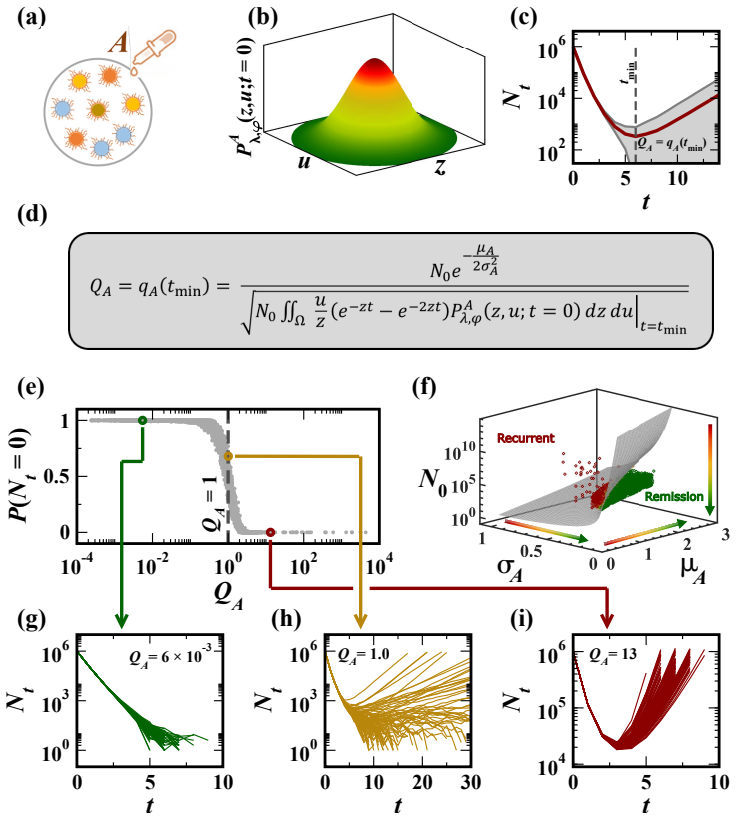
The paper's central claim is that the classic exponential-decay law $N_t=N_0 e^{-\lambda t}$ is replaced, for a heterogeneous population, by $N_A(t)=N_0 e^{K_\lambda(-t)}$, where $K_\lambda$ is the cumulant generating function of the initial per-cell net rate $\lambda=r_- - r_+$. The expected trajectory alone is incomplete: the variance $V_A(t)$ is computed from the joint distribution of $\lambda$ and $\varphi=r_-+r_+$, and the observable quantity that decides treatment success is $q_A(t)=N_A(t)/\sqrt{V_A(t)}$. Treatment $A$ succeeds when $Q_A=\min_t q_A(t)\leq 1$, and its duration is the first time $T_A$ at which this crossing happens. With rates drawn from a distribution whose lower edge is $\lambda_{\min}$, the asymptotic classes are exponential remission ($\lambda_{\min}>0$), slow remission ($\lambda_{\min}=0$, $N_A\sim t^{-\alpha}$, $T_A\sim N_0^{1/(1+\alpha)}$), and recurrence ($\lambda_{\min}<0$); even in the recurrent class, extinction by fluctuation can precede the rebound whenever the dip falls within one standard deviation of zero. Thus the outcome of treatment is determined by the shape of the response distribution—especially its tail and variance—not by its mean.
Load-bearing premise
The load-bearing premise is that each cell's birth and death rates are fixed when treatment begins and are inherited without mutation by daughter cells; if rates can change during treatment, the predicted classes, the $Q_A$ crossing, and the scaling of $T_A$ all lose their footing.
Editorial extensions
If this is right
- Treatment ranking by the mean decay rate alone will sometimes pick the wrong drug: a higher-variance treatment can look better in the first days and then reverse into recurrence, an effect observed in the data.
- In the slow-remission class, increasing the initial population size from $10^3$ to $10^7$ cells stretches the predicted cure time from tens to thousands of time units, so large tumors in this class have no bounded treatment duration.
- A treatment whose expected trajectory is recurrent can still be successful if, at its minimum, $N_A(t)$ is within one fluctuation width of zero; the $Q_A$ statistic separates these benign recurrent cases from dangerous ones.
- Measuring the initial distribution of per-cell rates, not just the average, becomes a clinically actionable step: it feeds directly into $Q_A$ and $T_A$.
Reading between the lines
- Beyond the paper: short-term single-cell tracking could estimate $P^A_\lambda(z;0)$ directly and rank drugs by $Q_A$ before long trials; this is a concrete translational route the authors only gesture at.
- The mutation-free assumption means the three classes are fixed at $t=0$; if resistance or adaptation changes rates during treatment, the power-law exponent and the $Q_A=1$ boundary should shift, and serial-passage experiments could test that shift.
- The crossover effect suggests that combined treatments with matched means but different variances may behave non-additively—an interaction the paper does not analyze, but which follows from its Eq. (7).
- A sharper experimental target: engineered clonal populations with Gamma-distributed rates should show median extinction times scaling as $N_0^{1/(1+\alpha)}$; the paper validates this only with simulations, so a wet-lab check would be decisive.
Signed reviews
Editorial analysis
A structured set of objections, weighed in public.
Referee Report
Summary. The paper develops a stochastic birth–death framework for heterogeneous cell populations in which each cell is assigned birth/death rates at t=0 and passes them to offspring without mutation. The main analytic results are Eq. (5), expressing the mean trajectory NA(t) as N0 exp[Kλ(−t)] with Kλ the cumulant generating function of the rate distribution; the asymptotic classification in Eq. (10) into exponential, slow, and recurrent remission based on the edge of Pλ; and the variance-based statistics qA, QA, TA in Eqs. (13)–(15), proposed as predictors of extinction probability and treatment duration. For Gamma-distributed slow-remission populations the theory yields TA ∼ N0^{1/(1+α)}, which the simulations in Fig. 4 confirm. The empirical section fits Eq. (7) to 78 cancer-cell trajectories with two parameters per trajectory.
Significance. The work addresses a real and important problem—treatment response in heterogeneous cell populations—and offers a compact analytic description that goes beyond the mean decay rate. Eq. (5) is correct for the stated model and unifies several known limits. The simulation tests in Fig. 4 are convincing: the scaling of NA, VA, qA, and the observed extinction times match the theory with apparently no free parameters beyond the chosen α. The crossover effect in Fig. 3k–m is an interesting consequence. However, the central extinction criterion QA≤1 is introduced as an ansatz rather than derived, and the empirical validation in Fig. 3 uses per-trajectory fitted parameters, so the paper's clinical claims are stronger than the evidence provided. With corrections and a clearly stated scope, the framework would be a valuable contribution.
major comments (6)
- [Section 'Population extinction - the role of VA(t)', Eqs. (13)-(15)] The extinction criterion QA≤1 is stated without derivation from P(Nt=0). The sharp transition in Fig. 5e supports it numerically for the normal and Gamma families, but no analytic link is supplied, so the criterion remains an ansatz whose accuracy for other rate distributions is unknown. Please derive (or at least heuristically justify) the connection between qA(t) and the hitting probability, and state the conditions under which it is expected to hold.
- [Section 'Modeling heterogeneous population dynamics', near Eq. (4)] The model explicitly assumes mutation-free inheritance: 'birth/death are stochastic, but the reproduction itself is mutation-free.' All predictions—the three classes, the QA crossing, and the scaling TA∼N0^{1/(1+α)}—are conditional on the initial rate distribution being frozen. Since the abstract and discussion frame the results for tumors under chemotherapy, where de novo resistance can arise during treatment, the central claim does not currently apply to the stated application. Please either add a model extension with rare rate-changing mutations and test whether the QA and TA predictions are robust, or explicitly restrict the clinical claims to the mutation-free regime.
- [Section 'Classes of population dynamics', Eq. (8)] The representation of Pλ as a power series in (z−λmin) with arbitrary real powers Ψn is introduced as 'quite generally' valid, but many densities (e.g., those vanishing faster than any power, or with logarithmic edge behavior) do not admit such an expansion. This expansion is the basis of Eq. (10) and of the three-class classification, so it is load-bearing. Please state the required regularity condition explicitly—for instance, Pλ(z) ∼ C0 (z−λmin)^{Ψ0} with Ψ0>−1—and note that the classification applies to this class of distributions.
- [Section 'The expected trajectory NA(t)', Eq. (12)] The variance formula in Eq. (12) is unreadable as printed: it contains an integral sign with no limits, and the integrand depends on t without an integration variable. Since VA(t) enters the defining statistic qA(t), the correct closed-form expression (or a pointer to the exact derivation in the Supplementary) must be provided in the main text.
- [Section 'The expected trajectory NA(t)', Fig. 3e-g] The empirical validation of Eq. (7) relies on fitting two free parameters (μi, σi) to each of the 78 trajectories; the collapse in Fig. 3g therefore does not constitute a parameter-free prediction. Please add a cross-validation scheme (e.g., fit on the early part of each trajectory and predict the late part) and report uncertainty or goodness-of-fit measures so the reader can judge predictive power.
- [Section 'Treatment success and efficiency', Eq. (17)] The printed scaling qA(t) ∼ sqrt(N0) t^{−α−1} is inconsistent with the preceding lines and with Eq. (18): from NA∼N0 t^{−α} and VA∼N0 t^{1−α} one obtains qA=NA/sqrt(VA) ∼ sqrt(N0) t^{−(α+1)/2}, which is what yields TA∼N0^{1/(1+α)} and matches Fig. 4i. Please correct the exponent in Eq. (17).
minor comments (2)
- [Section 'Population extinction - the role of VA(t)', Eq. (3)] The statement that Nt is 'likely to fall within' NA±√VA is a one-standard-deviation heuristic; please clarify that this is an approximation for the typical fluctuation and not a rigorous confidence interval.
- [Section 'Treatment success and efficiency', Fig. 4h caption] The caption in Fig. 4h refers to a 'striking agreement' but does not provide quantitative statistics (e.g., slope, R², or mean absolute error) for the TObs versus TA comparison; please add a summary statistic to support the claim.
Circularity Check
Empirical validations in Figs. 3g and 4h are partially self-fulfilling, but the core cumulant-based derivation and the slow-remission scaling Eq. (18) are self-contained.
-
fitted input called prediction
[Section 'Long-term behavior of NA(t)', Fig. 3e-g]
"To systematically test prediction (7) across the entire dataset, we extracted the best-fitting µi, σ2i for all 78 trajectories (i = 1,...,78). Namely, we fit the ith experiment to the predicted curve ni(t) = Ni(t)/Ni0 = efi(t), where fi(t) = −µit + σ2i t2/2. In Fig. 3g we collapse all data points by plotting ni(t) vs. fi(t), which according to our predicted (7) should follow a linear plot."
The two parameters µi and σi are fitted separately to each trajectory, so fi is chosen to make ni(t) ≈ e^{fi(t)} for that same curve. Consequently, the collapse of ni(t) versus fi(t) onto the line ni = e^{fi} is an identity that restates the fit rather than an independent confirmation that Eq. (7) predicts the trajectories. The analytic derivation of Eq. (7) from Eq. (5) is self-consistent, but the empirical claim that the 78 diverse responses are matched by a 'single universal function' is weaker than presented because the universal curve is not parameter-free: each trajectory contributes its own fitted µi and σi.
-
other
[Section 'Efficiency', Fig. 4h]
"We then compare this observed elimination time to our predicted TA in Eq. (15). Plotting T Obs A vs. TA across all 4,400 scenarios, we find a striking agreement, demonstrating the predictive power of our condition (15) to capture the actual timescales for treatment success (Fig. 4h). [Fig. 4h caption:] The observed extinction time T Obs A vs. the predicted TA in Eq. (15) as evaluated using the dashed line intersection of panel (f)."
In this comparison, the 'predicted' TA is not computed from the analytic formulas alone; it is read off the simulation-measured qA(t) shown in panel (f), i.e. from the very same stochastic ensembles that produce T_Obs_A. Comparing a statistic extracted from a curve to another statistic of the same curve-generating process is a self-consistency check, not an independent out-of-sample test. The analytic slow-remission scaling TA ∼ N0^{1/(1+α)}, derived from the predicted q in Eq. (17), is tested separately in Fig. 4i and is not affected by this issue; nevertheless, the paper's claim of predictive power for Eq. (15) relies in part on this same-data comparison.
full rationale
The central derivation is mathematically self-contained: Eq. (4) is the exact mean of the assumed mutation-free birth-death process with distributed rates, Eq. (5) is simply the cumulant generating function representation of that mean, and Eqs. (8)-(11) follow from an asymptotic expansion of the Laplace-type integral. The slow-remission scalings in Eq. (17) and Eq. (18) are parameter-free predictions given the assumed Gamma distribution, and they are validated in Fig. 4i against independently simulated median extinction times across six orders of magnitude of N0; that part is not circular. The recurrent-class boundary QA ≤ 1 is also tested against the fraction of extinction events in simulations implementing the same model, which is an internal consistency test but one that could in principle have failed. No load-bearing self-citation was found: the cited 'mutation-free' assumption is an explicit modeling choice stated in the text, and supporting references are not used to forbid alternatives. The two flagged issues are validation circularities in supporting empirical demonstrations: the normal-distribution data collapse of Fig. 3g is built from per-trajectory two-parameter fits, and the Fig. 4h agreement compares T_Obs to a TA evaluated from the same simulated q curves. These do not undermine the analytic derivation of the main classes or the independent scaling test in Fig. 4i, so the overall circularity score is moderate rather than high. The paper's mutation-free premise is a scope limitation for real tumors, not a circularity, because the model states it openly and all predictions are derived from it rather than assuming the conclusion.
Assumptions & free parameters
free parameters (1)
- mu_i and sigma_i per empirical trajectory =
e.g., mu=0.34, sigma=0.11; mu=0.17, sigma=0.04; mu=0.29, sigma=0.12 (Fig. 3f)
assumptions (3)
- domain assumption Each cell lineage follows a linear birth-death process with rates r+ and r-, and rates are inherited unchanged upon replication.
- ad hoc to paper The lambda-density can be expanded as a power series around a finite lambda_min with possibly negative or non-integer powers, as in Eq. (8).
- ad hoc to paper Extinction likelihood is controlled by qA(t) = NA(t)/sqrt(VA(t)), with q<=1 marking probable extinction.
Cite this review
Pith. "Pith review of Efficient treatment of heterogeneous malignant cell populations." pith.science (2026). https://pith.science/paper/FJT3BB2Y
@misc{pith2026250112691,
  author       = {Pith},
  title        = {Pith review of: Efficient treatment of heterogeneous malignant cell populations},
  year         = {2026},
  howpublished = {\url{https://pith.science/paper/FJT3BB2Y}},
  note         = {Machine review of arXiv:2501.12691}
}
read the original abstract
When confronted with an undesired cell population, such as bacterial infections or tumors, we seek the most effective treatment, designed to eliminate the population as rapidly as possible. A common practice is to monitor the cells short-term response to the treatment, and from that, extrapolate the eventual treatment outcome, i.e. will it eradicate the cells, and if yes at what timescales. Underlying this approach is the assumption that the cells exhibit a homogeneous response to the treatment, and hence the early response patterns can be naturally extended to later times. Recent experiments on cancer cell populations, however, indicate a significant level of cellular heterogeneity, undermining this classic assessment protocol of treatment efficacy. We, therefore, develop here a stochastic framework, to analytically predict the temporal dynamics of a heterogeneous cell population. Quite often, we find, the average cellular parameters, governing the short-term response, fail to predict the actual treatment outcome. In contrast, our analysis, which also incorporates the populations variability, helps identify the relevant statistical parameters, which in turn, enable us to predict the full trajectory of the cell population, and specifically - the likelihood and typical timescales for remission.
Figures


Figures from the paper (3 more)


Reference graph
Works this paper leans on
-
[1]
Individuality and slow dynamics in bacterial growth homeostasis
Lee Susman, Maryam Kohram, Harsh Vashistha, Jeffrey T Nechleba, Hanna Salman, and Naama Brenner. Individuality and slow dynamics in bacterial growth homeostasis. Proceedings of the National Academy of Sciences, 115(25):E5679–E5687, 2018
work page 2018
-
[2]
Universal protein distributions in a model of cell growth and division
Naama Brenner, CM Newman, Dino Osmanovi´ c, Yitzhak Rabin, Hanna Salman, and DL Stein. Universal protein distributions in a model of cell growth and division. Physical Review E , 92(4):042713, 2015
work page 2015
-
[3]
Rapid evolutionary adaptation to growth on an ‘unfamiliar’carbon source
Zvi Tamari, Avihu H Yona, Yitzhak Pilpel, and Naama Barkai. Rapid evolutionary adaptation to growth on an ‘unfamiliar’carbon source. BMC genomics , 17(1):1–7, 2016
work page 2016
-
[4]
Modeling cell population dynamics.In Silico Biology, 13(1-2):21–39, 2019
Daniel A Charlebois and G´ abor Bal´ azsi. Modeling cell population dynamics.In Silico Biology, 13(1-2):21–39, 2019
work page 2019
-
[5]
A note on birth–death processes with catastrophes
Antonio Di Crescenzo, Virginia Giorno, Amelia G Nobile, and Luigi M Ricciardi. A note on birth–death processes with catastrophes. Statistics & probability letters , 78(14):2248–2257, 2008
work page 2008
-
[6]
On a class of birth-death processes with time-varying intensity functions
Virginia Giorno and Amelia G Nobile. On a class of birth-death processes with time-varying intensity functions. Applied Mathematics and Computation , 379:125255, 2020
work page 2020
-
[7]
Nicolas Baca¨ er.A short history of mathematical population dynamics , volume 618. Springer, 2011
work page 2011
-
[8]
Persister cells and tolerance to antimicrobials
Iris Keren, Niilo Kaldalu, Amy Spoering, Yipeng Wang, and Kim Lewis. Persister cells and tolerance to antimicrobials. FEMS microbiology letters , 230(1):13–18, 2004
work page 2004
Show all 46 references
-
[9]
Bacterial persistence as a phenotypic switch
Nathalie Q Balaban, Jack Merrin, Remy Chait, Lukasz Kowalik, and Stanislas Leibler. Bacterial persistence as a phenotypic switch. Science, 305(5690):1622–1625, 2004
2004
-
[10]
Definitions and guidelines for research on antibiotic persistence
Nathalie Q Balaban, Sophie Helaine, Kim Lewis, Martin Ackermann, Bree Aldridge, Dan I Andersson, Mark P Brynildsen, Dirk Bumann, Andrew Camilli, James J Collins, et al. Definitions and guidelines for research on antibiotic persistence. Nature Reviews Microbiology, 17(7):441–448, 2019
2019
-
[11]
Persistence of antibiotic resistant bacteria
Dan I Andersson. Persistence of antibiotic resistant bacteria. Current opinion in microbiology, 6(5):452–456, 2003
2003
-
[12]
Evolutionary causes and consequences of bacterial antibiotic persistence
Erik Bakkeren, M´ ed´ eric Diard, and Wolf-Dietrich Hardt. Evolutionary causes and consequences of bacterial antibiotic persistence. Nature Reviews Microbiology, 18(9):479–490, 2020
2020
-
[13]
Cancer progression as a learning process
Aseel Shomar, Omri Barak, and Naama Brenner. Cancer progression as a learning process. Iscience, page 103924, 2022
2022
-
[14]
Distinguishing between resistance, tolerance and persistence to antibiotic treatment
Asher Brauner, Ofer Fridman, Orit Gefen, and Nathalie Q Balaban. Distinguishing between resistance, tolerance and persistence to antibiotic treatment. Nature Reviews Microbiology, 14(5):320–330, 2016
2016
-
[15]
Treatment of staphyloeoeeal infections with penicillin by intermittent sterilisation
JosephW Bigger et al. Treatment of staphyloeoeeal infections with penicillin by intermittent sterilisation. Lancet, pages 497–500, 1944
1944
-
[16]
Binomial moment equations for stochastic reaction systems
Baruch Barzel and Ofer Biham. Binomial moment equations for stochastic reaction systems. Physical Review Letters, 106(15):150602, 2011
2011
-
[17]
Stochastic analysis of complex reaction networks using binomial moment equations
Baruch Barzel and Ofer Biham. Stochastic analysis of complex reaction networks using binomial moment equations. Physical Review E , 86(3):031126, 2012
2012
-
[18]
Description of transient processes in multiplying medium by the physical birth-and-death model
MV Bobkova, TN Korbut, and Ed A Rudak. Description of transient processes in multiplying medium by the physical birth-and-death model. In Journal of Physics: Conference Series , volume 1689, page 012016. IOP Publishing, 2020
2020
-
[19]
Short-term forecast in the early stage of the covid- 19 outbreak in italy
Nicola Bartolomeo, Paolo Trerotoli, and Gabriella Serio. Short-term forecast in the early stage of the covid- 19 outbreak in italy. application of a weighted and cumulative average daily growth rate to an exponential decay model. Infectious Disease Modelling , 6:212–221, 2021
2021
-
[20]
Cancer cell population growth kinetics at low densities deviate from the exponential growth model and suggest an allee effect
Kaitlyn E Johnson, Grant Howard, William Mo, Michael K Strasser, Ernesto ABF Lima, Sui Huang, and Amy Brock. Cancer cell population growth kinetics at low densities deviate from the exponential growth model and suggest an allee effect. PLoS biology, 17(8):e3000399, 2019
2019
-
[21]
Determination of the decay rate of nitrifying bacteria
S Salem, MS Moussa, and MCM Van Loosdrecht. Determination of the decay rate of nitrifying bacteria. Biotechnology and bioengineering, 94(2):252–262, 2006. 18
2006
-
[22]
On the generalized” birth-and-death” process
David G Kendall. On the generalized” birth-and-death” process. The annals of mathematical statistics , 19(1):1–15, 1948
1948
-
[23]
Robust growth of escherichia coli
Ping Wang, Lydia Robert, James Pelletier, Wei Lien Dang, Francois Taddei, Andrew Wright, and Suckjoon Jun. Robust growth of escherichia coli. Current biology, 20(12):1099–1103, 2010
2010
-
[24]
IRS1 phosphorylation underlies the non-stochastic probability of cancer cells to persist during EGFR inhibition therapy
A Jacob Berger, E Gigi, L Kupershmidt, Z Meir et al. IRS1 phosphorylation underlies the non-stochastic probability of cancer cells to persist during EGFR inhibition therapy. Nature Cancer, 2:1055–1070, 2021
2021
-
[25]
On relaxations and aging of various glasses
Ariel Amir, Yuval Oreg, and Yoseph Imry. On relaxations and aging of various glasses. Proceedings of the National Academy of Sciences , 109(6):1850–1855, 2012
2012
-
[26]
Stochastic processes in physics and chemistry , volume 1
Nicolaas Godfried Van Kampen. Stochastic processes in physics and chemistry , volume 1. Elsevier, 1992
1992
-
[27]
Stochastic models of population extinction
Otso Ovaskainen and Baruch Meerson. Stochastic models of population extinction. Trends in ecology & evolution, 25(11):643–652, 2010
2010
-
[28]
Virus population extinction via ecological traps
John J Dennehy, Nicholas A Friedenberg, Yul W Yang, and Paul E Turner. Virus population extinction via ecological traps. Ecology Letters, 10(3):230–240, 2007
2007
-
[29]
Observation of universal ageing dynamics in antibiotic persistence
Yoav Kaplan, Shaked Reich, Elyaqim Oster, Shani Maoz, Irit Levin-Reisman, Irine Ronin, Orit Gefen, Oded Agam, and Nathalie Q Balaban. Observation of universal ageing dynamics in antibiotic persistence. Nature, 600(7888):290–294, 2021
2021
-
[30]
Random boolean network models and the yeast transcriptional network
Stuart Kauffman, Carsten Peterson, Bj¨ orn Samuelsson, and Carl Troein. Random boolean network models and the yeast transcriptional network. Proceedings of the National Academy of Sciences , 100(25):14796– 14799, 2003
2003
-
[31]
Slow relaxation and aging phenomena at the nanoscale in granular materials
VY Zaitsev, VE Gusev, Vincent Tournat, and Patrick Richard. Slow relaxation and aging phenomena at the nanoscale in granular materials. Physical review letters , 112(10):108302, 2014
2014
-
[32]
Estimation for general birth-death processes
Forrest W Crawford, Vladimir N Minin, and Marc A Suchard. Estimation for general birth-death processes. Journal of the American Statistical Association , 109(506):730–747, 2014
2014
-
[33]
Stochastic processes in cell biology , volume 41
Paul C Bressloff. Stochastic processes in cell biology , volume 41. Springer, 2014
2014
-
[34]
Computational methods for birth-death processes
Forrest W Crawford, Lam Si Tung Ho, and Marc A Suchard. Computational methods for birth-death processes. Wiley Interdisciplinary Reviews: Computational Statistics , 10(2):e1423, 2018
2018
-
[35]
Aging and death in an organism that reproduces by morphologically symmetric division
Eric J Stewart, Richard Madden, Gregory Paul, and Fran¸ cois Taddei. Aging and death in an organism that reproduces by morphologically symmetric division. PLoS biology, 3(2):e45, 2005
2005
-
[36]
Epidemic spreading under mutually independent intra- and inter-host pathogen evolution
Xiyun Zhang, Zhongyuan Ruan, Muhua Zheng, Jie Zhou, Stefano Boccaletti, and Baruch Barzel. Epidemic spreading under mutually independent intra- and inter-host pathogen evolution. Nature Communications, ”In print”, 2022
2022
-
[37]
H. Hahn. ¨Uber die nichtarchimedischen Gr¨ oßensysteme. In Hans Hahn Gesammelte Abhandlungen Band 1/Hans Hahn Collected Works Volume 1 , pages 445 – 499. Springer, 1995
1995
-
[38]
hipa, a newly recognized gene of escherichia coli k-12 that affects frequency of persistence after inhibition of murein synthesis
Harris S Moyed and Kevin P Bertrand. hipa, a newly recognized gene of escherichia coli k-12 that affects frequency of persistence after inhibition of murein synthesis. Journal of bacteriology , 155(2):768–775, 1983
1983
-
[39]
Characterization of the hipa7 allele of es- cherichia coli and evidence that high persistence is governed by (p) ppgpp synthesis
Shaleen B Korch, Thomas A Henderson, and Thomas M Hill. Characterization of the hipa7 allele of es- cherichia coli and evidence that high persistence is governed by (p) ppgpp synthesis. Molecular microbiology, 50(4):1199–1213, 2003
2003
-
[40]
Bacterial persistence: a model of survival in changing environments
Edo Kussell, Roy Kishony, Nathalie Q Balaban, and Stanislas Leibler. Bacterial persistence: a model of survival in changing environments. Genetics, 169(4):1807–1814, 2005
2005
-
[41]
Hidden killers: persistence of opportunistic fungal pathogens in the human host
Christophe d’Enfert. Hidden killers: persistence of opportunistic fungal pathogens in the human host. Current Opinion in Microbiology , 12(4):358–364, 2009
2009
-
[42]
Persistent candidemia in neonatal care units: risk factors and clinical significance
Majeda S Hammoud, Abdullah Al-Taiar, Mervat Fouad, Aditiya Raina, and Ziauddin Khan. Persistent candidemia in neonatal care units: risk factors and clinical significance. International Journal of Infectious Diseases, 17(8):e624–e628, 2013
2013
-
[43]
Finitely generated cumulants
Giovanni Pistone and Henry P Wynn. Finitely generated cumulants. Statistica Sinica, pages 1029–1052, 1999. 19
1999
-
[44]
Geometric constraints during epithelial jamming
Lior Atia, Dapeng Bi, Yasha Sharma, Jennifer A Mitchel, Bomi Gweon, Stephan A Koehler, Stephen J DeCamp, Bo Lan, Jae Hun Kim, Rebecca Hirsch, et al. Geometric constraints during epithelial jamming. Nature physics, 14(6):613–620, 2018
2018
-
[45]
Persistent heterogeneity not short-term overdispersion determines herd immunity to covid-19
Alexei V Tkachenko, Sergei Maslov, Ahmed Elbanna, George N Wong, Zachary J Weiner, and Nigel Gold- enfeld. Persistent heterogeneity not short-term overdispersion determines herd immunity to covid-19. arXiv preprint arXiv:2008.08142, 10(2020.07):26–20162420, 2020
2008 arXiv
-
[46]
Hogg and A.T
R.V. Hogg and A.T. Craig. Introduction to Mathematical Statistics (4th ed.) . Macmillan, New York, 1978. 20 Figures - Full size 𝑪 𝒓+, 𝒓_ 𝒓𝟎, 𝒓𝟎 𝑵𝒕 = 𝟒 𝑵𝒕 = 𝟑 𝑵𝒕 = 𝟐 𝑵𝒕 = 𝟏 𝑵𝒕 = 𝟎Treatment success 𝒓+ 𝒓𝟎 𝒓− Time 𝑵𝒕 𝓝𝑨(𝒕) 𝓥𝑨(𝒕) Time Real. 1 Real. 2 Real. 3𝓝 𝒕 = 𝒆−𝝀𝒕 (a) Expectati...
1978
Reviewed August 10, 2026 · model on record in the stance chip above.
Discussion (0). Continue with ORCID to comment.