REVIEW 3 major objections 6 minor 1 cited by
Tackling artefacts in the timing of relativistic pulsar binaries: towards the SKA
T0 review · 3 major / 6 minor · reviewed 2026-08-10 · deepseek-v4-flash
Pith's one-line read The Double Pulsar's orbital dispersion-measure variation was an artefact of neglecting the Doppler-shifted spin frequency during de-dispersion; the same approximations will bias Shapiro-delay measurements for tight edge-on binaries.
desk verdict A clean, likely-correct Doppler explanation for the Double Pulsar's 20-year-old DM artefact; the SKA-era Shapiro-bias claim in Section 6 is the part that needs harder scrutiny. read the letter →
The pith
A machine-rendered reading of the paper's core claim, the machinery that carries it, and where it could break.
The reading
What carries the argument
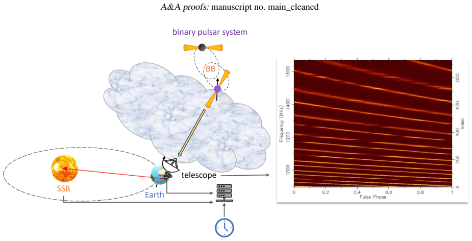
The load-bearing object is the one-dimensional polynomial phase predictor used in folding. Instead of evaluating the exact de-dispersed phase $\phi(t,f)=\phi^{(1)}(t-\Delta t_{\rm DM}[t,f,f_0];f_0)$, current software computes $\tilde{\phi}(t,f)\simeq\phi^{(1)}(t;f_0)-\nu^{(1)}(t_{\rm mid};f_0)\,\Delta t_{\rm DM}(t_{\rm mid},f,f_0)$, using a single reference frequency $f_0$ and a single mid-sub-integration epoch for the whole band. The key identity derived from this mismatch is $\delta\mathrm{DM}=\left(\sqrt{(1-\beta)/(1+\beta)}-1\right)\mathrm{DM}_0\simeq-\beta\,\mathrm{DM}_0$, which converts the neglected orbital Doppler factor into an apparent phase-dependent DM. For the second-order effects, the Taylor expansion of the phase predictor produces $\Delta\phi(t,f)=\Delta t_{\rm DM}[\ddot{\phi}_0\,\Delta t-\tfrac12\dddot{\phi}_0\,\Delta t^2+\cdots]-\tfrac12\Delta t_{\rm DM}^2[\ddot{\phi}_0+\dddot{\phi}_0\Delta t+\cdots]+\cdots$, whose leading term grows with sub-integration length (TDDS) and whose next term grows toward low frequency (SDDS). The Shapiro-delay failure is diagnosed by comparing the exact logarithmic delay $\Delta_S^{(\rm LO)}=-2r\ln\Lambda_u$ with the polynomial expansion used by standard predictors.
What would settle it
Re-process the original Green Bank Telescope observations behind the reported Double Pulsar DM curve with the full binary ephemeris, so the dispersive-phase correction uses the Doppler-shifted spin frequency at each orbital phase; the artefact interpretation predicts the apparent DM curve collapses to a constant $\mathrm{DM}_0$, whereas any surviving orbital modulation of order $0.05\,\mathrm{pc\,cm^{-3}}$ would indicate a real propagation component.
Extended reading notes
Core claim
On the paper's own terms, the central discovery is that the apparent orbital DM modulation attributed to plasma propagation is, at dominant order, exactly what you get by equating the true dispersive phase shift—computed with the Doppler-shifted observed spin frequency $\nu(t)=\nu_0\sqrt{(1-\beta)/(1+\beta)}$—with a 'solitary-pulsar' correction that uses the fixed spin frequency $\nu_0$. The result is an apparent DM offset $\delta\mathrm{DM}\simeq -\beta\,\mathrm{DM}_0 = -(v_r/c)\,\mathrm{DM}_0$, which for PSR J0737−3039A peaks near $0.05\,\mathrm{pc\,cm^{-3}}$ and traces the line-of-sight orbital velocity, matching the reported curve. The paper then identifies two second-order artefacts from assuming the spin frequency is constant over the sub-integration time (temporal dispersive Doppler smearing, TDDS) and over the band (spectral dispersive Doppler smearing, SDDS): both cause orbital-phase-dependent dispersive smearing that mimics DM variation, with magnitudes set by radial acceleration and the dispersive delay, and with eccentricity controlling the waveform. Finally, the paper shows that the polynomial phase predictors used in standard folding cannot represent the sharp logarithmic Shapiro delay for edge-on binaries with periods below about four hours, leaving spiky timing residuals at superior conjunction that bias the measured Shapiro range and shape parameters.
Load-bearing premise
The load-bearing premise is that current pulsar pipelines actually fold with a one-dimensional polynomial phase predictor evaluated at a single reference frequency and a single mid-sub-integration time across the whole band, so that the orbital Doppler shift really is neglected during de-dispersion.
Editorial extensions
If this is right
- De-dispersing before any time-averaging removes both TDDS and SDDS, so the orbital smearing artefacts disappear by changing only the order of data-processing steps.
- At SKA-Low frequencies, SDDS dominates for sub-integrations shorter than about half the dispersive delay (38 s for the Double Pulsar parameters), giving smearing of order 10 ms for a 1-hour orbit and 100 ms for a 15-minute orbit; at SKA-Mid, TDDS instead dominates once the sub-integration exceeds about 0.6 s.
- For edge-on binaries with orbital periods under roughly four hours, current polynomial predictors leave spiky residuals centred at superior conjunction; these residuals grow as the predictor's time span and the sub-integration length grow, and they bias the Shapiro range and shape parameters—estimated at about 2σ at the SKA's final configuration—even when statistical noise is tiny.
- Enabling the barycentric correction for the dispersive delay removes the apparent annual DM modulation, whose maximum relative amplitude is about $10^{-4}$ for pulsars near the ecliptic plane.
Reading between the lines
- If the DDV interpretation is correct, previously published orbital DM variations in other relativistic binaries should be re-checked: the missed Doppler shift predicts a specific phase curve tied to the line-of-sight velocity, so matching that curve is not by itself evidence of a real electron-column change.
- A cheap, testable extension is to look for the same artefact in any strongly accelerated pulsar—for example in a globular cluster—processed with one-dimensional predictors; the predicted apparent DM curve follows the radial velocity and should be reproducible without new physics.
- The Shapiro-delay folding failure points to a concrete software design target: add the analytic logarithmic Shapiro term directly to the phase model, or move to a two-dimensional phase predictor, rather than trying to fit the cusp with more polynomial coefficients.
Editorial analysis
A structured set of objections, weighed in public.
Referee Report
Summary. This paper investigates signal-processing artefacts in pulsar timing of relativistic binaries, focusing on the Double Pulsar PSR J0737-3039A. The authors first show that the apparent orbital DM variation reported by Ransom et al. (2004) can be explained as a dispersive Doppler variation (DDV): neglecting the Doppler-shifted spin frequency when computing the dispersive phase shift produces an apparent DM offset δDM ≈ -(v_r/c) DM0 (Eq. 9), with amplitude about 0.05 pc cm^-3, matching the reported value. They then derive and simulate two second-order effects, temporal and spectral dispersive Doppler smearing (TDDS and SDDS), and show that these also cause orbital-phase-dependent apparent DM variations. The paper additionally considers topocentric analogues of these effects and argues that polynomial phase predictors (polyco) fail to accurately model the sharp logarithmic Shapiro delay for edge-on orbits with periods below about 4 hours, leading to potentially significant biases in Shapiro-delay parameter measurements with sensitive instruments such as FAST and the SKA.
Significance. The DDV explanation is a clean, parameter-free derivation with a concrete numerical prediction that matches an external observation, and the paper correctly distinguishes this first-order effect from the second-order smearing effects TDDS and SDDS, which have been repeatedly confused in the literature. The scaling relations in Eqs. (14) and (15) and the summary table are useful practical tools for observers, and the proposed mitigation (de-dispersion before frequency or time averaging) is actionable. The section on topocentric artefacts is a welcome extension. However, the SKA/Shapiro-delay bias claim is less convincing: the simulations in Section 6 appear to use the same polynomial approximation for both generation and folding, so the residuals shown in Figs. 15-17 and the bias estimates in Table 2 do not independently test the predictor against the exact timing model. This weakens a central claim for the future-SKA part of the paper, although the underlying mathematical concern about polynomial representation of the logarithmic Shapiro delay is well founded.
major comments (3)
- [Section 6, Fig. 15 and Table 2] The simulations used to demonstrate the Shapiro-delay/polyco problem are not an independent test because PsrSigSim generates the pulsar data files 'based on the polynomial expansion of the timing solution (predictor)', as stated in Section 6. If generation and folding use the same polyco coefficients (or the same TZNSPAN/coefficient set), the residuals in Figs. 15-17 show only the inconsistency between two uses of the same approximation, not the error relative to the exact timing model. The paper does not specify whether the generator used an exact tempo/tempo2 ephemeris and a high-resolution predictor, or whether generation and folding share the same approximation. Thus the simulated bias estimates in Table 2, and the claim that polynomial predictors will bias Shapiro-delay measurements at SKA sensitivity, are not supported by the current simulations. The authors should regenerate these simulations with an exact-ephemeris forward model (generating pulse times from the full DD model with the Shapiro logarithmic term) and then fold with polyco, so that the difference directly quantifies the predictor error.
- [Section 2, Eq. (3) and Section 4.1] The premise that current pipelines (dspsr, psrchive, presto) use the one-dimensional phase approximation of Eq. (3), applying a polynomial evaluated at one reference frequency and one mid-sub-integration time across the whole band, is load-bearing for all three artefacts (DDV, TDDS, SDDS). This is asserted on page 3 but not documented with code-level references or a concrete audit. Please provide a brief but explicit description of where each package makes this approximation (e.g., the relevant function or configuration), or state clearly which default settings are assumed. Without this, the reader cannot judge whether the predicted artefact amplitudes apply to the actual software used by the community, including the handling of the barycentric correction discussed in Section 5.
- [Section 4.2.1, Fig. 9 and surrounding text] The claim that the apparent DM variation from TDDS for the Double Pulsar is 'consistent with what has been seen with MeerKAT when processing the data in a similar fashion' is not quantified. Because the TDDS amplitude is an order of magnitude smaller than the DDV and because the variation depends on profile shape and orbital eccentricity, a visual comparison alone is insufficient. Please provide a quantitative comparison, such as the best-fit amplitude and the residual chi-squared or RMS between the simulated and observed DM variations for the same orbital phase bins, or clearly label the statement as a qualitative similarity.
minor comments (6)
- [Section 4.1, Eq. (6)] The symbol used for the radial velocity of the pulsar appears as '3psr r (t)' in the text; this is not defined and is confusing. Please write it as v_psr^r(t) or a similar standard notation and define it at first use.
- [Section 4.2.1, Eq. (11) and surrounding text] The derivative notation using the symbols ':' and ';' (e.g., 'ϕ0' and ':ϕ0') is non-standard and not explained. Please replace with conventional dot notation (e.g., dϕ/dt, d²ϕ/dt²) or define the notation explicitly near Eq. (11).
- [Section 5.1, Eq. (16)] The definition 'where D = D× DM' uses the same symbol D for the dispersion constant and the product D×DM. Please use a distinct symbol for the product to avoid ambiguity.
- [Section 6, first paragraph after Table 1] The phrase 'the discrepancies of interest should be visible in the residuals after subtracting the best-fit timing model' relies on the underlying generator using the same predictor; this should be clarified earlier in the section, as noted in Major Comment 1, so that the reader is not misled about the independence of the test.
- [References] The reference for Ransom et al. (2004) is given as an arXiv eprint (astro-ph/0406321). Since the paper is described as having been withdrawn, please provide the withdrawal status and any associated comment or erratum in the reference list or a footnote, so interested readers can locate the original and the retraction.
- [Abstract and Section 7] The abstract states that the polynomial approximation fails for 'orbits less than 4 hours', but the simulations in Fig. 15 were run for 4.5 h, 3 h, 2.45 h, and 1 h, so the 4-hour threshold is an interpolation between the simulated points. Please state this explicitly or add a simulation at a period just above and below 4 hours to justify the threshold.
Circularity Check
No significant circularity: the analytic derivations are parameter-free and the simulations forward-model the stated approximations, benchmarked against external data.
full rationale
The paper's central DDV claim follows algebraically by equating the dispersive phase computed with the Doppler-shifted spin frequency (Eq. 6) and with the rest-frequency spin (Eq. 7), yielding Eq. (9); this is a closed-form consequence, not a fitted parameter. The comparison with Ransom et al. (2004) is external, using the known orbital velocity and DM0 of PSR J0737-3039A rather than values adjusted to match the reported DM curve. The TDDS/SDDS expressions (Eqs. 13-15 and 18-19) are Taylor expansions of the difference between Eqs. (3) and (4), and the associated simulations are consistency checks of those analytic formulae, not inversions in which the target result is used as input. Section 6's Shapiro-delay bias estimates do rely on PsrSigSim generating phase-connected data via a polyco polynomial, as the text explicitly notes; however, this is a controlled injection of the predictor error into synthetic TOAs followed by a fit to the exact timing model, so the reported biases in s and r are a nontrivial propagation of that error rather than a restatement of the input. The self-citation to Hu et al. (2022) supplies the Double Pulsar ephemeris and a prior qualitative mention of the folding issue, but the present paper's derivations and external benchmarks do not reduce to that citation.
Assumptions & free parameters
free parameters (3)
- Synthetic orbital periods used in folding tests =
1, 3, 4.5 hours
- Synthetic orbital eccentricities in smearing tests =
0.0, 0.088, 0.6
- Phase-predictor resolution (TZNSPAN, coefficient count) =
1-3 minutes, 20-30 coefficients
assumptions (5)
- domain assumption The cold-plasma dispersion relation with delay t_DM = D x DM / f^2 is the correct description of dispersion in the interstellar medium and in pulsar software.
- domain assumption The current processing chain folds data with a one-dimensional phase predictor evaluated at a single reference frequency and mid-sub-integration time, as in Eq. (3).
- standard math Taylor expansions of the phase predictor in Eqs. (11)-(13) converge over the sub-integration and bandwidth used in the simulations.
- standard math The Shapiro delay formula from Blandford and Teukolsky (1976), Eqs. (20)-(21), is the correct timing-model description that the polynomial predictor approximates.
- domain assumption The simulated PSR J0737-3039A ephemeris and template profile from Hu et al. (2022) are accurate enough to reproduce the real processing artefacts.
Cite this review
Pith. "Pith review of Tackling artefacts in the timing of relativistic pulsar binaries: towards the SKA." pith.science (2026). https://pith.science/paper/C4CB2TSZ
@misc{pith2026250116421,
  author       = {Pith},
  title        = {Pith review of: Tackling artefacts in the timing of relativistic pulsar binaries: towards the SKA},
  year         = {2026},
  howpublished = {\url{https://pith.science/paper/C4CB2TSZ}},
  note         = {Machine review of arXiv:2501.16421}
}
read the original abstract
Common signal-processing approximations produce artefacts when timing pulsars in relativistic binary systems, especially edge-on systems with tight orbits, such as the Double Pulsar. In this paper, we use extensive simulations to explore various patterns that arise from the inaccuracies of approximations made when correcting dispersion and Shapiro delay. In a relativistic binary, the velocity of the pulsar projected onto the line-of-sight varies significantly on short time scales, causing rapid changes in the apparent pulsar spin frequency, which is used to convert dispersive delays to pulsar rotational phase shifts. A well-known example of the consequences of this effect is the artificial variation of dispersion measure (DM) with binary phase, first observed in the Double Pulsar 20 years ago. We show that ignoring the Doppler shift of the spin frequency when computing the dispersive phase shift exactly reproduces the shape and magnitude of the reported DM variations. We also simulate and study two additional effects of much smaller magnitude, which are caused by the assumption that the spin frequency used to correct dispersion is constant over the duration of the sub-integration and over the observed bandwidth. We show that failure to account for these two effects leads to orbital phase-dependent dispersive smearing that leads to apparent orbital DM variations. The functional form of the variation depends on the orbital eccentricity. In addition, we find that a polynomial approximation of the timing model is unable to accurately describe the Shapiro delay of edge-on systems with orbits less than 4 hours, which poses problems for the measurements of timing parameters, most notably the Shapiro delay. This will be a potential issue for sensitive facilities like the FAST and the forthcoming Square Kilometre Array (SKA); therefore, a more accurate phase predictor is indispensable.
Figures

Figures from the paper (11 more)


Forward citations
Cited by 1 Pith paper
-
Unlocking Gravity and Gravitational Waves with Radio Pulsars: Advances and Challenges
This review summarizes pulsar-based gravity tests and updates simulations predicting that the Double Pulsar will yield a neutron star moment of inertia measurement to about 5% by 2038.
Reference graph
Works this paper leans on
-
[1]
& Teukolsky, S
Blandford, R. & Teukolsky, S. A. 1976, ApJ, 205, 580
1976
-
[2]
Breton, R. P., Kaspi, V . M., Kramer, M., et al. 2008, Science, 321, 104
work page 2008
-
[3]
Burgay, M., D’Amico, N., Possenti, A., et al. 2003, Nature, 426, 531
work page 2003
-
[4]
Cameron, A. D., Champion, D. J., Kramer, M., et al. 2018, MNRAS, 475, L57
work page 2018
-
[5]
Damour, T. & Deruelle, N. 1986, Annales de l’institut Henri Poincaré (A) Physique théorique, 44, 263
work page 1986
-
[6]
1915, Sitzungsberichte der Königlich Preussischen Akademie der Wissenschaften, 844
Einstein, A. 1915, Sitzungsberichte der Königlich Preussischen Akademie der Wissenschaften, 844
work page 1915
-
[7]
Freire, P. C. C. & Wex, N. 2024, Living Reviews in Relativity, 27, 5
2024
-
[8]
Hazboun, J. S. & Shapiro-Albert, B. 2020, Pulsar Data Toolbox
work page 2020
Show all 31 references
-
[9]
B., Edwards, R
Hobbs, G. B., Edwards, R. T., & Manchester, R. N. 2006, MNRAS, 369, 655
2006
-
[10]
W., van Straten, W., & Manchester, R
Hotan, A. W., van Straten, W., & Manchester, R. N. 2004, PASA, 21, 302
2004
-
[11]
2023, PhD thesis, University of Bonn
Hu, H. 2023, PhD thesis, University of Bonn
2023
-
[12]
& Freire, P
Hu, H. & Freire, P. C. C. 2024, Universe, 10, 160
2024
-
[13]
J., et al
Hu, H., Kramer, M., Champion, D. J., et al. 2022, A&A, 667, A149
2022
-
[14]
J., & Kehl, M
Hu, H., Kramer, M., Wex, N., Champion, D. J., & Kehl, M. S. 2020, MNRAS, 497, 3118
2020
-
[15]
Hulse, R. A. & Taylor, J. H. 1975, ApJ, 195, L51
1975
-
[16]
M., Ransom, S
Kaspi, V . M., Ransom, S. M., Backer, D. C., et al. 2004, ApJ, 613, L137
2004
-
[17]
H., Manchester, R
Kramer, M., Stairs, I. H., Manchester, R. N., et al. 2006, Science, 314, 97
2006
-
[18]
H., Manchester, R
Kramer, M., Stairs, I. H., Manchester, R. N., et al. 2021, Physical Review X, 11, 041050
2021
-
[19]
Lorimer, D. R. & Kramer, M. 2004, Handbook of Pulsar Astronomy, V ol. 4
2004
-
[20]
E., Kramer, M., Shannon, R
Lower, M. E., Kramer, M., Shannon, R. M., et al. 2024, A&A, 682, A26
2024
-
[21]
G., Burgay, M., Kramer, M., et al
Lyne, A. G., Burgay, M., Kramer, M., et al. 2004, Science, 303, 1153
2004
-
[22]
Manchester, R. N. & Taylor, J. H. 1972, Astrophys. Lett., 10, 67
1972
-
[23]
2015, Tempo: Pulsar timing data analysis, Astrophysics Source Code Library, record ascl:1509.002 Özel, F
Nice, D., Demorest, P., Stairs, I., et al. 2015, Tempo: Pulsar timing data analysis, Astrophysics Source Code Library, record ascl:1509.002 Özel, F. & Freire, P. 2016, ARA&A, 54, 401
2015
-
[24]
M., Backer, D
Ransom, S. M., Backer, D. C., Demorest, P., et al. 2004, arXiv eprint [arXiv:astro-ph/0406321]
2004 arXiv
-
[25]
Shapiro, I. I. 1964, Phys. Rev. Lett., 13, 789
1964
-
[26]
J., Hazboun, J
Shapiro-Albert, B. J., Hazboun, J. S., McLaughlin, M. A., & Lam, M. T. 2021, Astrophys. J., 909, 219
2021
-
[27]
Stovall, K., Freire, P. C. C., Chatterjee, S., et al. 2018, ApJ, 854, L22
2018
-
[28]
H., Fowler, L
Taylor, J. H., Fowler, L. A., & McCulloch, P. M. 1979, Nature, 277, 437
1979
-
[29]
Taylor, J. H. & Weisberg, J. M. 1982, ApJ, 253, 908
1982
-
[30]
Taylor, J. H. & Weisberg, J. M. 1989, ApJ, 345, 434 van Straten, W. & Bailes, M. 2011, PASA, 28, 1
1989
-
[31]
& Kramer, M
Wex, N. & Kramer, M. 2020, Universe, 6, 156 Article number, page 13 of 13
2020
Reviewed August 10, 2026 · model on record in the stance chip above.
Discussion (0). Continue with ORCID to comment.