REVIEW 3 major objections 5 minor 23 references
Continuity-Preserving Convolutional Autoencoders for Learning Continuous Latent Dynamical Models from Images
T0 review · 3 major / 5 minor · reviewed 2026-08-09 · deepseek-v4-flash
Pith's one-line read The paper proves that Lipschitz-smooth convolutional filters keep latent states from image frames continuous enough for a Neural ODE to model.
desk verdict Useful diagnosis and a regularizer that works in practice, but the main theorem's proof only covers small translations; the paper is still worth citing and refereeing. read the letter →
The pith
A machine-rendered reading of the paper's core claim, the machinery that carries it, and where it could break.
The reading
What carries the argument
The load-bearing object is the filter-smoothness condition: writing discrete filter weights as samples $W_l(j\delta)$ of a function $W_l$, the encoder is $\delta$-continuous when $W_l$ is Lipschitz. The proof uses the translation invariance and weight sharing of convolutions to shift the evaluation grid $Y^l$ along with the object, reducing a pixel motion $\Delta$ to differences $W_l(\cdot+\Delta)-W_l(\cdot)$; large early filters $J_l=O(1/\delta)$ make the translation term decay as $2^{-(L^*-1)}$. The regularizer in Eq. (6), borrowed from nonlocal image processing, penalizes squared differences of nearby filter weights with a Gaussian kernel and is applied to the first three layers in the CpAE architecture.
What would settle it
Train CpAE on a translating object whose path crosses the image border; if the latent states still show per-step changes bounded by a constant times the time step, Assumption 3.1 is unnecessary, while if jumps appear exactly at boundary contact, the premise is what carries the result.
Extended reading notes
Core claim
The central claim is Theorem 3.1. For rigid-body planar motion, under an assumption that the object's feature support stays away from the image boundary, if the filter functions $W_l$ in the first $L^*$ layers satisfy $|W_l(y_1)-W_l(y_2)| \le c_W \|y_1-y_2\|$ and strides are 2, then the encoder composition $E^\delta \circ I^\delta \circ S$ is $\delta$-continuous: for small pixel size $\delta$, $\|E^\delta(I^\delta(S(z_1)))-E^\delta(I^\delta(S(z_2)))\| \le C c_W \|z^r_1-z^r_2\| + C c_W 2^{-(L^*-1)} \|z^t_1-z^t_2\|$ as $\delta \to 0$. Thus rotation enters with a full Lipschitz constant while translation is damped by the number of early layers. The paper argues that standard CNN filters, being arbitrary arrays of weights, violate this condition and therefore make latent trajectories discontinuous, and that promoting filter smoothness with Eq. (6) restores it.
Load-bearing premise
The load-bearing premise is that the moving object stays inside a central region of the image, away from the boundary, so that a shifted convolution grid coincides with the original grid; the proof's bound depends on that coincidence, and separately on trained filter weights behaving like samples of a fixed smooth function as resolution increases.
Editorial extensions
If this is right
- Latent states produced by a CpAE satisfy $\|Z_{n+1}-Z_n\| \le c_E M_f \Delta t$, so they are discrete samples of a Lipschitz trajectory and can be modeled by a Neural ODE.
- CpAE improves Valid Prediction Time and Valid Prediction Frequency over standard autoencoders on damped pendulum, elastic pendulum, double pendulum, and swing stick benchmarks.
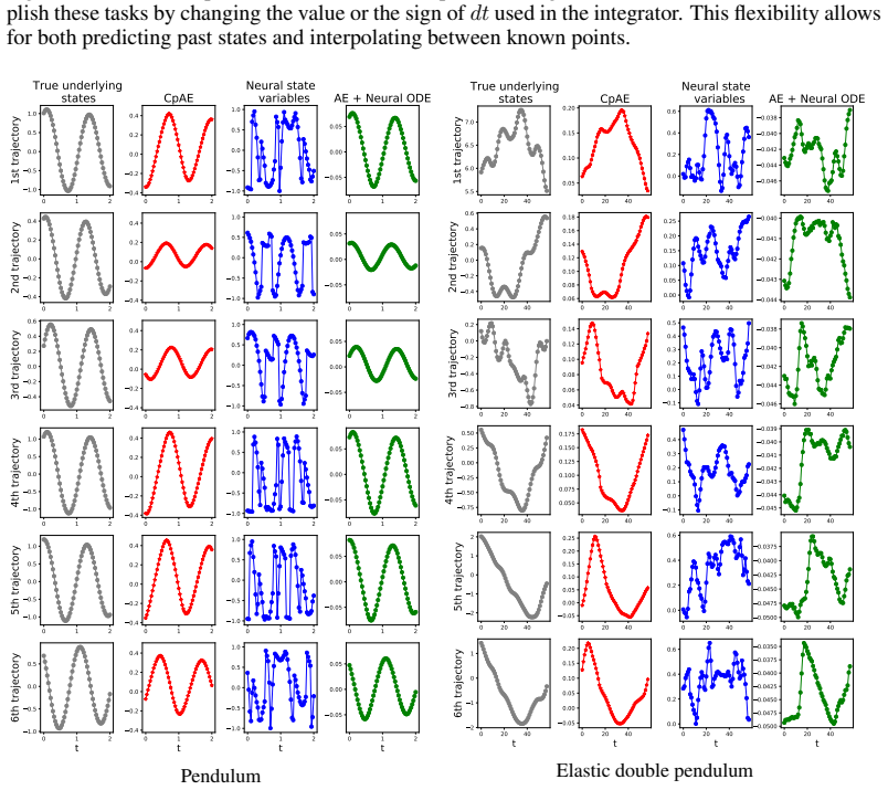
- Because the latent model is continuous, the same trained model can predict backward in time and interpolate between observed frames by integrating with negative or intermediate time steps.
- Filter size must scale with resolution ($J_l = O(1/\delta)$) in the first $L^*$ layers; the paper uses $12\times 12$ filters on $128\times 256$ images with $L^*=4$.
- The regularizer weight $\lambda_J$ trades off reconstruction fidelity against latent continuity; too large a weight underfits, too small reintroduces jumps.
Reading between the lines
- Extension: the theorem's translation term decays as $2^{-(L^*-1)}$, suggesting that deeper early stacks with large filters should tame translation-induced jumps even further, at higher memory cost; the paper does not sweep $L^*$.
- Extension: because Assumption 3.1 fails when the object reaches the image border, CpAE's advantage should degrade exactly on trajectories with boundary contact; measuring latent jump size as a function of distance to the border would isolate the mechanism.
- Extension: the same regularizer could be applied to Vision Transformers, whose patch operations are convolutions with kernel equal to patch size; a direct test would be whether patch-based encoders with smooth patch weights also yield continuous latent series.
- Extension: the regularity criterion suggests a diagnostic: before fitting any latent ODE, inspect the filter Lipschitz constants of the trained encoder; small constants predict trustworthy continuity, large ones predict the standard-AE failure mode.
Editorial analysis
A structured set of objections, weighed in public.
Referee Report
Summary. The paper proposes continuity-preserving convolutional autoencoders (CpAEs) for learning latent dynamical models from image frames. It introduces a δ-continuity relaxation of Lipschitz continuity, argues that standard CNN encoders can produce latent states that jump between adjacent frames, and proves a sufficient condition (Theorem 3.1) under which rigid-body motion in 2D yields δ-continuous latent states when the first L* convolution filters are Lipschitz. The proposed method adds a nonlocal regularization term (Eq. (6)) to promote filter continuity and trains a Neural ODE on the resulting latent states. Experiments on circular motion, damped/elastic pendulums, double pendulum, and swing stick show improved valid prediction time compared with autoencoders coupled with Neural ODE, HNN, or SympNets.
Significance. If Theorem 3.1 can be established as stated, the paper makes a useful conceptual contribution: it formalizes why pixel discretization breaks naive continuity assumptions, gives a checkable sufficient condition (filter Lipschitzness) for latent-state continuity, and demonstrates a simple regularizer with consistent empirical gains. The authors are also appropriately explicit about limitations, including the restriction to 2D rigid-body motion and the degraded performance on swing stick. However, the central theorem currently has a proof gap in the translational part of the bound, and the connection between the asymptotic theorem and the fixed-resolution experiments rests on idealizations that are not enforced by the training loss. These issues are load-bearing for the paper's main claim.
major comments (3)
- [Appendix A.2.3, Corollary A.3] The proof of the translational bound applies Assumption A.1 to the recursive shifts and asserts that Y^l − (Δ̂^{l+1}_k − Δ̂^l_k) = Y^l 'due to Assumption A.1'. Assumption A.1 only guarantees this grid equivalence for shifts with ‖Δ‖∞ ≤ M∆, where M∆ is the central-region margin. The recursive increments are differences of binary remainders of the total translation and can have norm comparable to the total translation; for example, with L=4 and a translation of 16δ, the first recursive increment is 16δ, which exceeds any small margin M∆, while a non-vacuous central-region condition requires M∆ < 1/2. Consequently, Theorem 3.1 is not proven for arbitrary pairs z1,z2 ∈ Z; as written, it covers only translations of size O(M∆) unless M∆ is taken so large that Assumption 3.1 fails for any object of nonzero area. Because the translational term is exactly the part of the bound that the continuity regularizer is intended to control, this gap needs to be repaired, for example by restricting the theorem to per-frame translations bounded by M∆ or by replacing Assumption A.1 with a stronger condition that is actually verified in the experiments.
- [Section 3.4 and Appendix A.2.1] Theorem 3.1 is an asymptotic statement as δ→0 in which the discrete filters W^δ_l are point samples of a fixed Lipschitz function W_l independent of δ, and J_l = O(1/δ). The experiments use fixed 128×128 images with finite 12×12 filters, and Eq. (6) is only a soft penalty on filter differences at that single resolution. Nothing in the training procedure guarantees the existence of a fixed Lipschitz function whose samples are the trained weights, so the theorem does not directly certify the continuity observed in the experiments. Please state this idealization as a limitation or provide a non-asymptotic bound that applies at the resolutions actually used.
- [Assumption 3.1 / Section 5] The theorem requires all feature maps to vanish outside a central region [M∆,1−M∆]^2 for every state in Z. For trajectories such as the swing-stick dataset, where objects approach or cross the image boundary, this premise is not satisfied; the authors themselves report a decline in performance on this task. The paper should discuss whether Assumption 3.1 can be verified for each benchmark and, if not, separate the theoretical claim from the empirical demonstration on those datasets.
minor comments (5)
- [Section 3.5 versus Section 4] The encoder description in Section 3.5 says images are of size 3×128×256, while the experiments in Sections 4.2 and 4.3 repeatedly state 3×128×128; please reconcile this inconsistency.
- [Equation (6)] The summation limits in Eq. (6) are typeset as 'J l+ Ĵ X i1,i2,j1,j2=−Ĵ', which is ambiguous; the intended range over filter positions and the neighborhood Ĵ should be written explicitly.
- [Appendix A.3.1] The proof of Theorem 3.1 omits activation and normalization layers, but the actual encoder in Appendix A.3.1 uses ReLU and batch normalization after every convolutional layer. ReLU is Lipschitz, but the effect of batch normalization on the δ-continuity bound is not addressed; please clarify which layers are covered by the theorem.
- [Corollary A.3] The definition of l^*_{k,j} does not handle the case |I_{k,j}| = 0, for which no positive integer satisfies 2^{l^*-1} ≤ 0; the zero-translation components should be treated separately.
- [Section 4.2] There is a duplicated word in 'The images of the physical state maintain the form of a single pendulum and are are generated...'.
Circularity Check
No significant circularity: Theorem 3.1 is derived from explicit assumptions; self-citations are not load-bearing.
full rationale
The central claim is Theorem 3.1: if the first L* convolution filters are Lipschitz and Assumption 3.1 holds, then the latent states of a CNN autoencoder are delta-continuous for 2D rigid-body motion. This is a mathematical derivation from stated assumptions, not a fit to data: the proof in Appendix A.2 builds on a function representation of the CNN, translation invariance (Lemma A.1), and recursive shift estimates (Lemmas A.2 and A.3), with the final bound following from Corollary A.3. The regularizer in Eq. (6) is motivated by the theorem and is then evaluated on held-out trajectories; hyperparameters are tuned on validation, which is standard practice and not a disguised prediction. The author-overlap citations, VPNet (Zhu et al., 2022) and SympNets (Jin et al., 2020), are used as an empirical regularizer and as baselines, respectively, and the continuity guarantee does not depend on them; hence they are not load-bearing for the main result. The paper itself notes in Section 5 that the analysis is limited to rigid-body motion in 2D, and a technical gap may exist in Corollary A.3 where Assumption A.1 is applied to recursive shifts whose size is not obviously bounded by M_Delta; however, that is a soundness or scope concern, not a circular reduction. No equation is equivalent to its own input by construction, and no fitted parameter is renamed as a prediction. Therefore the appropriate circularity score is 0.
Assumptions & free parameters
free parameters (5)
- λJ (continuity regularizer weight) =
1 by default; ablated in Fig. 15
- λR (VPNet orientation-preservation weight) =
1 by default; ablated in Fig. 15
- σ (Gaussian kernel width in Eq. (6)) =
not specified
- VPT threshold ε =
0.007 for first three datasets; 0.0015 for swing stick
- Filter size Jl and number of continuity layers L* =
Jl = 12, L* = 4
assumptions (7)
- domain assumption The underlying dynamical system f is Lipschitz continuous and bounded by Mf.
- domain assumption Image formation is a noiseless binary occupancy discretization Iδ(S(z)) of a state-to-set map S.
- domain assumption Motion is rigid-body translation plus rotation in 2D with pairwise disjoint objects (Eqs. 4-5).
- ad hoc to paper Assumption 3.1: feature-map support is confined to a central image region away from boundaries.
- ad hoc to paper Filter weights Wl are normalized to a fixed bounded Lipschitz function Wl on R2 independent of δ, with discrete filters as point samples.
- domain assumption Volume-preserving maps ΦΔ exist for rigid motion with ||ΦΔ(x) - x|| ≤ c1 ||Δ||.
- ad hoc to paper Omitted operations such as activation layers do not change continuity.
Cite this review
Pith. "Pith review of Continuity-Preserving Convolutional Autoencoders for Learning Continuous Latent Dynamical Models from Images." pith.science (2026). https://pith.science/paper/AHKQD3I3
@misc{pith2026250200754,
  author       = {Pith},
  title        = {Pith review of: Continuity-Preserving Convolutional Autoencoders for Learning Continuous Latent Dynamical Models from Images},
  year         = {2026},
  howpublished = {\url{https://pith.science/paper/AHKQD3I3}},
  note         = {Machine review of arXiv:2502.00754}
}
read the original abstract
Continuous dynamical systems are cornerstones of many scientific and engineering disciplines. While machine learning offers powerful tools to model these systems from trajectory data, challenges arise when these trajectories are captured as images, resulting in pixel-level observations that are discrete in nature. Consequently, a naive application of a convolutional autoencoder can result in latent coordinates that are discontinuous in time. To resolve this, we propose continuity-preserving convolutional autoencoders (CpAEs) to learn continuous latent states and their corresponding continuous latent dynamical models from discrete image frames. We present a mathematical formulation for learning dynamics from image frames, which illustrates issues with previous approaches and motivates our methodology based on promoting the continuity of convolution filters, thereby preserving the continuity of the latent states. This approach enables CpAEs to produce latent states that evolve continuously with the underlying dynamics, leading to more accurate latent dynamical models. Extensive experiments across various scenarios demonstrate the effectiveness of CpAEs.
Figures


Figures from the paper (12 more)




Reference graph
Works this paper leans on
-
[2]
For the other datasets, a latent state dimension of 8 was used. These values are intentionally larger than the theoretical minimum to enhance the model’s expressiveness. CNN autoencoder . The architecture of CNN encoder in this paper is adapted from the setting provided by Chen et al. (2022). The encoder is a 16-layer CNN, with the parameters of the down-...
work page 2022
-
[4]
Samuel Greydanus, Misko Dzamba, and Jason Yosinski. Hamiltonian neural networks. In 33rd Conference on Neural Information Processing Systems (NeurIPS 2019), pp. 15353–15363,
work page 2019
-
[6]
Diederik P. Kingma and Max Welling. Auto-encoding variational bayes. In 2nd International Conference on Learning Representations (ICLR 2014),
work page 2014
-
[7]
Deep lagrangian networks: Using physics as model prior for deep learning
Michael Lutter, Christian Ritter, and Jan Peters. Deep lagrangian networks: Using physics as model prior for deep learning. In 7th International Conference on Learning Representations (ICLR 2019). OpenReview.net,
work page 2019
-
[8]
Resnet after all: Neural ODEs and their numerical solution
Katharina Ott, Prateek Katiyar, Philipp Hennig, and Michael Tiemann. Resnet after all: Neural ODEs and their numerical solution. In 9th International Conference on Learning Representations (ICLR 2021),
work page 2021
-
[12]
We employ a very small VPNet for regularization
VPNet. We employ a very small VPNet for regularization. It comprises three linear layers, each consisting of two sublayers. The activation function employed is Sigmoid. Neural ODE. Neural Ordinary Differential Equations (Neural ODE) Chen et al. (2018) are contin- uous models by embedding neural networks into continuous dynamical systems. In this paper, we...
work page 2018
-
[14]
Rezende, Andrew Jaegle, S ´ebastien Racani `ere, Aleksandar Botev, and Irina Higgins
Peter Toth, Danilo J. Rezende, Andrew Jaegle, S ´ebastien Racani `ere, Aleksandar Botev, and Irina Higgins. Hamiltonian generative networks. In 8th International Conference on Learning Repre- sentations (ICLR 2020). OpenReview.net,
work page 2020
-
[15]
Symmetry-Informed Governing Equation Discovery
Jianke Yang, Wang Rao, Nima Dehmamy, Robin Walters, and Rose Yu. Symmetry-informed gov- erning equation discovery. arXiv preprint arXiv:2405.16756,
Show all 23 references
-
[16]
Symplectic ode-net: Learning hamiltonian dynamics with control
Yaofeng Desmond Zhong, Biswadip Dey, and Amit Chakraborty. Symplectic ode-net: Learning hamiltonian dynamics with control. In 8th International Conference on Learning Representations (ICLR 2020). OpenReview.net,
2020
-
[17]
13 Published as a conference paper at ICLR 2025 A A PPENDIX A.1 R IGID MOTION MODELING Here we consider rigid body motion, namely that all its particles maintain the same distance relative to each other. The position of the whole body can be represented by the imaginary transl...
2025
-
[18]
15 Published as a conference paper at ICLR 2025 Given that maxl maxj1,j2 |ϕl(yl−1 1 , yl)|/(⌈Jl/2⌉δ) ≤ cϕ, we must choose Jl = O(1/δ)
Here C is a constant independent of δ and z. 15 Published as a conference paper at ICLR 2025 Given that maxl maxj1,j2 |ϕl(yl−1 1 , yl)|/(⌈Jl/2⌉δ) ≤ cϕ, we must choose Jl = O(1/δ). Under this choice, the normalization coefficients εl can be set as: ε1 = δ2/|S(z)|, εl = δ2 for l...
2025
-
[19]
Due to weight sharing, the convolution operation exhibits translational invariance
We can readily check that two equivalent evaluation sets yield equivalent results for the convolution operation, i.e., if Y l = ˆY l, Il+1(yl+1, z|Y l, Yl−1, · · ·, Y0) = Il+1(yl+1, z| ˆY l, Yl−1, · · ·, Y0). Due to weight sharing, the convolution operation exhibits translatio...
2025
-
[20]
Finally, applying Lemma A.3, we have aL(∆) ≤ L−1X i=0 M i ϕMI KX k=1 cϕ 2l∗ k,1−1 |∆k,1| + cϕ 2l∗ k,2−1 |∆k,2|
In addition, we have bl−i( ˆ∆l−i k − ˆ∆l−i−1 k ) =bl−i (il−i k,1 − il−i−1 k,1 )δ, (il−i k,2 − il−i−1 k,2 )δ =bl−i ⌊il−i k,1 /2l−i−1⌋ ·2l−i−1 δ, ⌊il−i k,2 /2l−i−1⌋ ·2l−i−1 δ ≤cϕ ⌊il−i k,1 /2l−i−1⌋ δ + cϕ ⌊il−i k,2 /2l−i−1⌋ δ ≤ cϕ 2l∗ k,1−1 |iL k,1|δ + cϕ 2l∗ k,2−1 |iL k,2|δ, wh...
2025
-
[22]
All convolutional layers are ac- companied by a batch normalization layer and a ReLU activation function
Each downsampling convolutional layer is followed by an additional convolutional layer with same number of output channels, but a 3 × 3 filter, a stride of 1, and zero padding of 1 to enhance expressiveness. All convolutional layers are ac- companied by a batch normalization l...
2025
-
[1985]
Distilling free-form natural laws from experimental data.Science, 324(5923):81–85,
12 Published as a conference paper at ICLR 2025 Michael Schmidt and Hod Lipson. Distilling free-form natural laws from experimental data.Science, 324(5923):81–85,
2025
-
[2009]
Auto-encoder based data clustering
Chunfeng Song, Feng Liu, Yongzhen Huang, Liang Wang, and Tieniu Tan. Auto-encoder based data clustering. In Progress in Pattern Recognition, Image Analysis, Computer Vision, and Appli- cations: 18th Iberoamerican Congress, CIARP 2013, pp. 117–124. Springer,
2013
-
[2016]
A brief review of hypernetworks in deep learning
Vinod Kumar Chauhan, Jiandong Zhou, Ping Lu, Soheila Molaei, and David A Clifton. A brief review of hypernetworks in deep learning. arXiv preprint arXiv:2306.06955,
-
[2018]
Unsupervised learning of invariant feature hierarchies with applications to object recognition
Marc’Aurelio Ranzato, Fu Jie Huang, Y-Lan Boureau, and Yann LeCun. Unsupervised learning of invariant feature hierarchies with applications to object recognition. In 2007 IEEE conference on computer vision and pattern recognition, pp. 1–8. IEEE,
2007
-
[2019]
Identification of dis- tributed parameter systems: A neural net based approach
11 Published as a conference paper at ICLR 2025 Raul Gonz ´alez-Garc´ıa, Ramiro Rico-Mart `ınez, and Ioannis G Kevrekidis. Identification of dis- tributed parameter systems: A neural net based approach. Computers & Chemical Engineering, 22:S965–S968,
2025
-
[2021]
Variational autoencoder for deep learning of images, labels and captions
Yunchen Pu, Zhe Gan, Ricardo Henao, Xin Yuan, Chunyuan Li, Andrew Stevens, and Lawrence Carin. Variational autoencoder for deep learning of images, labels and captions. In 30th Confer- ence on Neural Information Processing Systems (NIPS 2016),
2016
-
[2022]
Multistep neural networks for data- driven discovery of nonlinear dynamical systems
Maziar Raissi, Paris Perdikaris, and George Em Karniadakis. Multistep neural networks for data- driven discovery of nonlinear dynamical systems. arXiv preprint arXiv:1801.01236,
-
[2023]
Deep clustering with convolutional au- toencoders
Xifeng Guo, Xinwang Liu, En Zhu, and Jianping Yin. Deep clustering with convolutional au- toencoders. In Neural Information Processing: 24th International Conference, ICONIP 2017, Guangzhou, China, pp. 373–382. Springer,
2017
-
[2024]
Lagrangian neural networks
Miles Cranmer, Sam Greydanus, Stephan Hoyer, Peter Battaglia, David Spergel, and Shirley Ho. Lagrangian neural networks. arXiv preprint arXiv:2003.04630,
2003 arXiv
Reviewed August 9, 2026 · model on record in the stance chip above.
Discussion (0). Continue with ORCID to comment.