Estimating Probabilities of Causation with Machine Learning Models

Ang Li; Shuai Wang

REVIEW 3 major objections 6 minor 32 references

Estimating Probabilities of Causation with Machine Learning Models

T0 review · 3 major / 6 minor · reviewed 2026-08-07 · deepseek-v4-flash

Challenge this review Re-run · record.json Download PDF Read on arXiv ↗

Pith's one-line read An MLP with the Mish activation function predicts the bounds of the probability of necessity and sufficiency for 32,768 subpopulations with a mean absolute error of about 0.02, after training on about 2,000 subpopulations with sufficient…

desk verdict Plausible ML transfer-learning pilot for PNS bounds, but the 'first' claims are overstated and the missing train/test split makes the headline MAE unverifiable as stated. read the letter →

arxiv 2502.08858 v1 pith:PIEQ2DAS submitted 2025-02-13 cs.AI

Shuai Wang , Ang Li This is my paper · ORCID

classification cs.AI

keywords probabilitiesofcausationprobabilitynecessityandsufficiencyPNSboundscausalinferencemachinelearningpredictionmultilayerperceptronMishactivationfunctionsubpopulationswithinsufficientdata

verification ladder T0 review T1 audit T2 compute T3 formal

The pith

A machine-rendered reading of the paper's core claim, the machinery that carries it, and where it could break.

The reading

The paper tries to show that machine learning can estimate probabilities of causation, in particular the probability of necessity and sufficiency (PNS), for subpopulations whose own experimental and observational data are too sparse to compute those quantities directly. It proposes training a regression model on subpopulations that do have enough data, using their observed characteristics as features and their PNS bounds as labels. In a simulated structural causal model with 15 observed and 5 unobserved binary confounders, about 2,000 of the 32,768 possible subpopulations meet the data sufficiency threshold, and a multilayer perceptron with the Mish activation function predicts the PNS lower and upper bounds across all 32,768 subpopulations with mean absolute error around 0.02. If this holds, causal quantities that previously required roughly 1,300 experimental and observational samples per subgroup could be obtained for rare subgroups from population-level patterns alone.

What carries the argument

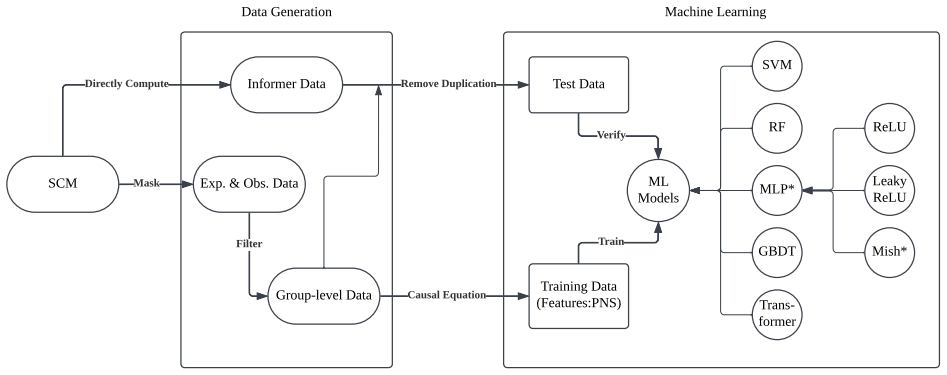
The carrying object is the tight bounds on PNS: the lower bound is the maximum of 0, $P(y_x)-P(y_{x'})$, $P(y)-P(y_{x'})$, and $P(y_x)-P(y)$, while the upper bound is the minimum of $P(y_x)$, $P(y_{x'})$, $P(x,y)+P(x',y')$, and $P(y_x)-P(y_{x'})+P(x,y')+P(x',y)$. The paper converts these formulas into regression labels: for each subpopulation it computes the experimental and observational distributions from the known structural causal model, plugs them into the bound equations, and trains models to map the 15 observed binary features to those labels. The best-performing configuration is a multilayer perceptron with layers 15, 64, 32, 16, and 1, using the Mish activation $s\cdot\tanh(\ln(1+e^s))$, a smooth non-monotonic function chosen because the PNS lower bound has many exact zeros and Mish remains differentiable at zero.

What would settle it

Recompute the true PNS bounds from the appendix's fixed structural causal model for the subpopulations that fell below the 1,300-sample threshold, and compare the MLP(Mish) predictions against those values; if the mean absolute error on that held-out rare-subpopulation slice is substantially above 0.02, the generalization claim is refuted.

Watch

Extended reading notes

Core claim

The center of the paper is a supervised regression claim: the pair of tight PNS bounds is a function of a subpopulation's observable characteristics, and that function can be learned from a subset of subpopulations that have enough data. The paper fixes a structural causal model, computes the true bounds for all $2^{15}$ observed feature combinations, filters out subpopulations with fewer than 1,300 experimental or observational samples, and trains five model classes on the remaining about 2,000 entries. The reported outcome is that an MLP with the Mish activation function reaches mean squared error 0.0011 on the lower bound and 0.0010 on the upper bound, and mean absolute error 0.0225 and 0.0247, substantially better than support vector regression, random forest, gradient boosting, and the Transformer. The authors take this as evidence that machine learning is a feasible tool for estimating probabilities of causation when direct estimation is impractical.

Load-bearing premise

The roughly 2,000 subpopulations that have at least 1,300 experimental and observational samples are representative of all 32,768 subpopulations, so a model trained only on them can predict bounds for the rare subpopulations it never sees.

Editorial extensions

If this is right

Subpopulation-level causal bounds can be obtained without collecting 1,300 experimental and observational samples for every subgroup, as long as some data-rich subgroups exist and share the same feature space.
The reported 0.02 mean absolute error suggests the learned bounds are accurate enough to rank subgroups by PNS, for example in unit-selection tasks that look for subgroups with high lower bounds or low upper bounds.
Because PN and PS have bounds of the same structural form, the same machine learning pipeline should extend to those probabilities, even though the experiments here report PNS only.
Model and activation choice matter: the smooth Mish activation outperforms ReLU and LeakyReLU on a target with many zero labels, indicating that tailoring the architecture to the causal quantity's shape is important.

Reading between the lines

Editorial extensions of the paper, not claims the author makes directly.

The method's success on one synthetic structural causal model suggests a broader amortized-identification principle: a neural network can internalize the mapping from population features to causal bounds, effectively compressing experimental and observational distributions into a feature lookup.
A stress test the paper does not run is to vary the number of unobserved confounders; as the gap between observed features and the true causal mechanism widens, the achievable accuracy should degrade, and the rate of degradation would tell practitioners how many confounders can safely be ignored.
For real deployments, true PNS bounds are unknown, so the practical version of this claim would be tested by collecting a small set of high-quality subgroups as a validation set and checking whether predicted bounds agree with directly computed bounds on those held-out groups.

Share X Bluesky LinkedIn Reddit HN

Editorial analysis

A structured set of objections, weighed in public.

Desk editor's note, referee report, and a circularity audit.

Desk Editor's Note

read the letter

Here's the short version: the paper's formulation—train ML models on subpopulations with enough data to estimate PNS bounds, then predict bounds for sparse subpopulations—is sound and worth a look. The execution is a single synthetic SCM, and the headline MAE of ~0.02 for MLP-Mish is plausible, but the evaluation protocol is under-specified enough that I can't verify it from the text alone.

What's genuinely there: the SCM is fully specified in the appendix, the code is released, and the comparison across five models and three activations is systematic. If you need a quick benchmark for this kind of transfer-learning framing, this is a reasonable starting point.

The soft spots are real but not fatal. First, the paper claims 'first ML pipeline for predicting probabilities of causation' in the contributions, yet it cites Li et al. 2022a,b as already demonstrating ML for this task. That's an overstatement you should fix. Second, the train/test split is never described. Section 4.3 says the training set has 2,054 (LB) and 2,065 (UB) entries after filtering, but the figures show ~30,713 points. The stress-test note observes that this is almost exactly 32,768 - 2,054 = 30,714, which would mean the evaluation is on the held-out complement—a genuine generalization test. But the abstract says 'for 32,768 subpopulations using data from around 2,000,' which sounds like training on 2,000 and evaluating on all 32,768. One sentence in the paper would resolve this, and it's currently missing. Third, the abstract says 'predicting PNS' but the models output bounds; the conclusion gets this right. Minor. Fourth, the training subpopulations are the data-rich ones, which could differ from rare subgroups, though the held-out complement result would mitigate that for this SCM.

My take: this is a useful pilot for people working at the causal-ML interface, but it's not a milestone. It deserves a serious referee if the authors clarify the split and moderate the novelty claims. The code and data generation make the work reproducible, which counts for a lot.

Referee Report

3 major / 6 minor

Summary. The paper proposes a supervised machine learning pipeline that predicts the Tian-Pearl bounds of the probability of necessity and sufficiency (PNS) for subpopulations whose own experimental and observational data are too sparse for direct estimation. The authors generate a synthetic structural causal model (SCM) with 15 observed and 5 unobserved binary features, compute exact PNS bounds for all 2^15 = 32,768 observed subpopulations from the SCM equations, and then train five models (SVM, random forest, GBDT, Transformer, and MLP with several activation functions) on the roughly 2,000 subpopulations that have at least 1,300 experimental and observational samples. The central claim is that an MLP with the Mish activation function achieves a mean absolute error of about 0.02 in predicting the PNS bounds across the 32,768 subpopulations, and the paper concludes that machine learning is a feasible tool for estimating probabilities of causation when subgroup-level data are insufficient.

Significance. If the claimed result holds as a genuine held-out generalization, the paper makes a useful feasibility contribution: it shows that a purely supervised map from observable subgroup features to causal-effect bounds can be learned from well-measured subpopulations and applied to poorly measured ones. The explicit SCM, the exact informer-data computation, the inclusion of code, and the comparison of several model families are strengths that make the result reproducible and testable. However, the significance is currently tempered by two issues: the evaluation protocol is under-specified, so the headline MAE is ambiguous, and the experiment is a single synthetic SCM with one fixed coefficient draw, so the external validity of the claim is unknown. The paper is best read as a proof-of-concept rather than a general claim about real-world probability-of-causation estimation.

major comments (3)

[Section 4.3] The train/test split is never stated. Section 4.3 reports 2,054 lower-bound and 2,065 upper-bound training entries, while the abstract claims an MAE of about 0.02 for 32,768 subpopulations. If the reported errors were computed on a set that includes the training subpopulations, the result would be optimistically biased and would not directly support the generalization claim. Notably, the confusion matrices in Figure 4 sum to about 30,713 (lower bound) and 30,702 (upper bound), which is very close to 32,768 minus 2,054 and 32,768 minus 2,065, respectively. This suggests that the evaluation was actually performed on the complement of the training subpopulations, i.e., on exactly the subpopulations with insufficient data. The paper must state this explicitly, report the MAE/MSE separately on the held-out complement, and clarify whether the reported 32,768 figure includes the training subpopulations. This is load-bearing for the central claim.
[Section 4.3 and Section 6] The training set is selected by requiring at least 1,300 experimental and observational samples per subpopulation, whereas the target population is subpopulations with insufficient data. The paper provides no analysis of the distribution shift between the training subpopulations and the test subpopulations, such as the range of features, the fraction of zero lower bounds, or the spread of PNS values in each group. If the held-out complement is indeed the test set, the reported MAE would already constitute an empirical answer for this SCM, but the paper should still describe the coverage of the training distribution and acknowledge the possibility that the learned map might not transfer to subpopulations outside the support of the training features. This is relevant to the generalization claim and should be addressed explicitly.
[Section 3 and Appendix A] The experimental evidence rests on a single SCM instance with one fixed draw of the coefficient vectors MX, MY, CY and one fixed set of Bernoulli parameters. The MLP(MLP-Mish) result is therefore a statement about this particular data-generating process, not about PNS prediction in general. The paper acknowledges in the Discussion that the causal structure is simple and that future work should consider more complex SCMs, which is appropriate. However, the conclusion that 'machine learning is a powerful tool for causal inference' goes beyond what a single configuration can support. I would ask the authors to either soften the conclusion to the specific SCM studied or add a small sensitivity analysis (e.g., multiple random SCM draws) to show that the MAE of about 0.02 is not an artifact of the chosen coefficients.

minor comments (6)

[Section 1.1] The paper states that 'no prior work has applied machine learning to the problem of predicting probabilities of causation', but the same introduction cites Li et al. [2022a,b] as demonstrating 'the potential of machine learning models to achieve accurate estimations for (sub)populations'. These claims should be reconciled to avoid an overstatement of novelty.
[Section 5.5] The MLP architecture is described as '15 → 64 → 32 → 16 → 1, utilizing ReLU-like functions and Sigmoid as activation functions', but the experiments compare ReLU, LeakyReLU, and Mish. Please specify which activation is used in each hidden layer and which is used at the output, and clarify how Mish fits the 'ReLU-like' description.
[Figures 3 and 4] The plots labeled 'confusion matrices' are joint histograms of binned true and predicted values for a regression task, not classification confusion matrices. Consider renaming them to 'prediction-error histograms' or 'agreement matrices' to avoid confusion.
[Section 4.3] The lower-bound data has 2,054 entries while the upper-bound data has 2,065 entries, even though both bounds are defined for the same subpopulations. Please explain this discrepancy; if it is due to a duplication-removal step or to subpopulations for which the bound is degenerate, state that explicitly.
[Abstract and Conclusion] The abstract and conclusion say the model predicts 'PNS' with an MAE of about 0.02, but the experiments actually predict the lower and upper bounds of PNS, not PNS itself. Rephrase to 'PNS bounds' for accuracy.
[Table 1] Table 1 reports point estimates of MSE and MAE without confidence intervals or repeated-run variance. Since the reported differences among models (e.g., MLP-ReLU vs MLP-LeakyReLU) are small, providing standard deviations over multiple seeds would strengthen the comparison.

Circularity Check

0 steps flagged · score 0.0 of 10

No significant circularity: PNS-bound prediction is a genuine supervised generalization task with labels computed from a fully specified SCM, not from the model inputs.

full rationale

The paper's derivation chain is a supervised regression from 15 observable subpopulation features to PNS bounds that are computed from a fully specified SCM with all coefficients and exogenous distributions given in the appendix. Training labels are derived from the SCM equations and are not used as inputs at test time, so the predictions are not fitted values renamed as predictions. The train/test separation is not explicitly described, but the confusion matrices sum to approximately 30,713 entries, matching the complement of the roughly 2,054 training subpopulations (32,768 - 2,054 = 30,714), which indicates that the reported MAE of about 0.02 is evaluated on held-out subpopulations with insufficient data. The mapping from observed features to PNS bounds is a well-defined deterministic function of the SCM and the distributions of the hidden variables, so learning that mapping from a subset of subpopulations is a genuine generalization task rather than a tautology. The paper cites prior work by the same authors for the SCM template and for the 1,300-sample adequacy heuristic, but those citations are not load-bearing for the numerical result because the SCM and all parameter values are fully specified in the paper itself. The absence of an explicit train/test split statement is a reporting ambiguity and a correctness risk, but it is not circular reasoning: no equation reduces to its own input, no fitted parameter is presented as a prediction, and no uniqueness claim is imported from the authors' prior work. The benchmark is self-generated, which limits external generalizability, but that is a limitation of scope, not circularity.

Assumptions & free parameters 4 free parameters · 4 assumptions · 0 invented entities

The central empirical result rests on the specific synthetic SCM, the filtering of training subpopulations by sample count, and the standard PNS bounds. The SCM coefficients and Bernoulli parameters are fixed inputs, not fitted to the target. The main unstated premise is the representativeness of the training subpopulations.

free parameters (4)

SCM coefficient vectors MX, MY and scalar CY = 20 coefficients each; CY = -0.7795 (Appendix A)
These coefficients define the synthetic data-generating process; the learnability of PNS bounds and the reported MAE depend on this particular SCM. They are randomly generated and fixed once, so they are inputs rather than fitted targets.
Bernoulli parameters for exogenous variables UZi, UX, UY = 22 probabilities listed in Appendix A
These determine the distribution over subpopulations and the observational/experimental distributions; they were randomly drawn from [0,1] and fixed.
MLP architecture and training hyperparameters = 15-64-32-16-1, Adam lr=0.01, 1000 epochs
Chosen by the authors; the Mish activation was selected after comparing on the test set, which is a model selection choice that affects the central result.
Minimum sample threshold for training subpopulations = 1,300
Subpopulations with fewer than 1,300 samples are excluded from training, which shapes the training distribution; the value comes from a cited paper but is a choice.

assumptions (4)

domain assumption For each subpopulation, the probabilities of causation are determined by the observed characteristics Z1,...,Z15.
Stated in the abstract; true in the synthetic SCM because the hidden features are independent and marginalized, but not guaranteed in real applications.
standard math The bounds for PNS, PS, PN from Tian and Pearl (2000) are correct and tight.
Used in Equations 1-6 to compute labels; this is established prior work.
domain assumption The selected subpopulations with sufficient samples are representative of all subpopulations.
Section 4.3 filters subpopulations by sample size; the paper does not test whether this selection is uninformative.
domain assumption A standard SCM with binary treatment/effect and exogenous Bernoulli noise captures the target setting.
Section 3 defines the SCM; results are only shown for this model.

how reviews work

0 comments

Cite this review

Pith. "Pith review of Estimating Probabilities of Causation with Machine Learning Models." pith.science (2026). https://pith.science/paper/PIEQ2DAS

@misc{pith2026250208858,
  author       = {Pith},
  title        = {Pith review of: Estimating Probabilities of Causation with Machine Learning Models},
  year         = {2026},
  howpublished = {\url{https://pith.science/paper/PIEQ2DAS}},
  note         = {Machine review of arXiv:2502.08858}
}

read the original abstract

Probabilities of causation play a crucial role in modern decision-making. This paper addresses the challenge of predicting probabilities of causation for subpopulations with insufficient data using machine learning models. Tian and Pearl first defined and derived tight bounds for three fundamental probabilities of causation: the probability of necessity and sufficiency (PNS), the probability of sufficiency (PS), and the probability of necessity (PN). However, estimating these probabilities requires both experimental and observational distributions specific to each subpopulation, which are often unavailable or impractical to obtain with limited population-level data. We assume that the probabilities of causation for each subpopulation are determined by its characteristics. To estimate these probabilities for subpopulations with insufficient data, we propose using machine learning models that draw insights from subpopulations with sufficient data. Our evaluation of multiple machine learning models indicates that, given sufficient population-level data and an appropriate choice of machine learning model and activation function, PNS can be effectively predicted. Through simulation studies, we show that our multilayer perceptron (MLP) model with the Mish activation function achieves a mean absolute error (MAE) of approximately 0.02 in predicting PNS for 32,768 subpopulations using data from around 2,000 subpopulations.

Figures

Figures reproduced from arXiv: 2502.08858 by the authors.

**Figure 2.** Comparison of true and predicted values across different models for both lower and upper bounds. [PITH_FULL_IMAGE:figures/full_fig_p005_2.png] view at source ↗

**Figure 3.** Confusion matrices of SVM, RF, GBDT, and Transformer models. [PITH_FULL_IMAGE:figures/full_fig_p006_3.png] view at source ↗

Figures from the paper (2 more)

**Figure 4.** Figure 4: Confusion matrices of MLP with different activation functions: ReLU, Leaky ReLU, and Mish for both lower and [PITH_FULL_IMAGE:figures/full_fig_p008_4.png]

**Figure 5.** Figure 5: Comparison of MLP (Mish) for lower and upper [PITH_FULL_IMAGE:figures/full_fig_p008_5.png]

Discussion (0). Continue with ORCID to comment.

Reference graph

Works this paper leans on

32 extracted references · 23 canonical work pages

[1]

Probabilistic counterfactuals: semantics, computation, and applications

Alexander Abraham Balke. Probabilistic counterfactuals: semantics, computation, and applications. University of California, Los Angeles, 1995

work page 1995
[2]

Random search for hyper-parameter optimization

James Bergstra and Yoshua Bengio. Random search for hyper-parameter optimization. Journal of machine learning research, 13 0 (2), 2012

work page 2012
[3]

Support-vector networks

Corinna Cortes. Support-vector networks. Machine Learning, 1995

1995
[4]

The probability of causation

Philip Dawid, Monica Musio, and Rossella Murtas. The probability of causation. Law, Probability and Risk, 16: 0 163--179, 2017

work page 2017
[5]

Friedman

Jerome H. Friedman. Greedy function approximation: A gradient boosting machine. Annals of Statistics, 29 0 (5): 0 1189--1232, 2001. doi:10.1214/aos/1013203451

arXiv 2001
[6]

An axiomatic characterization of causal counterfactuals

David Galles and Judea Pearl. An axiomatic characterization of causal counterfactuals. Foundations of Science, 3 0 (1): 0 151--182, 1998

work page 1998
[7]

Axiomatizing causal reasoning

Joseph Y Halpern. Axiomatizing causal reasoning. Journal of Artificial Intelligence Research, 12: 0 317--337, 2000

work page 2000
[8]

Causal analysis after haavelmo

James Heckman and Rodrigo Pinto. Causal analysis after haavelmo. Econometric Theory, 31 0 (1): 0 115--151, 2015

work page 2015

Show all 32 references

[9]

Random decision forests

Tin Kam Ho. Random decision forests. In Proceedings of 3rd international conference on document analysis and recognition, volume 1, pages 278--282. IEEE, 1995

1995
[10]

Causal inference in statistics, social, and biomedical sciences

Guido W Imbens and Donald B Rubin. Causal inference in statistics, social, and biomedical sciences. Cambridge university press, 2015

2015
[11]

Unit selection based on counterfactual logic

Ang Li and Judea Pearl. Unit selection based on counterfactual logic. In Proceedings of the Twenty-Eighth International Joint Conference on Artificial Intelligence, 2019

2019
[12]

Probabilities of causation: Role of observational data

Ang Li and Judea Pearl. Probabilities of causation: Role of observational data. In International Conference on Artificial Intelligence and Statistics, pages 10012--10027. PMLR, 2023

2023
[13]

Probabilities of causation with nonbinary treatment and effect

Ang Li and Judea Pearl. Probabilities of causation with nonbinary treatment and effect. In Proceedings of the AAAI Conference on Artificial Intelligence, volume 38, pages 20465--20472, 2024 a

2024
[14]

Unit selection with nonbinary treatment and effect

Ang Li and Judea Pearl. Unit selection with nonbinary treatment and effect. In Proceedings of the AAAI Conference on Artificial Intelligence, volume 38(18), pages 20473--20480, 2024 b

2024
[15]

Chen, Jingzheng Qin, and Zhen Qin

Ang Li, Suming J. Chen, Jingzheng Qin, and Zhen Qin. Training machine learning models with causal logic. In Companion Proceedings of the Web Conference 2020, pages 557--561, 2020

2020
[16]

Learning probabilities of causation from finite population data

Ang Li, Song Jiang, Yizhou Sun, and Judea Pearl. Learning probabilities of causation from finite population data. arXiv preprint arXiv:2210.08453, 2022 a

2022 arXiv
[17]

Unit selection: Learning benefit function from finite population data

Ang Li, Song Jiang, Yizhou Sun, and Judea Pearl. Unit selection: Learning benefit function from finite population data. In NeurIPS 2022 Workshop on Causality for Real-world Impact, 2022 b

2022
[18]

Probabilities of causation: Adequate size of experimental and observational samples

Ang Li, Ruirui Mao, and Judea Pearl. Probabilities of causation: Adequate size of experimental and observational samples. In NeurIPS 2022 Workshop on Neuro Causal and Symbolic AI (nCSI), 2022 c

2022
[19]

Rectifier nonlinearities improve neural network acoustic models

Andrew L Maas, Awni Y Hannun, Andrew Y Ng, et al. Rectifier nonlinearities improve neural network acoustic models. In Proc. icml, volume 30, page 3. Atlanta, GA, 2013

2013
[20]

Mish: A self regularized non-monotonic activation function

Diganta Misra. Mish: A self regularized non-monotonic activation function. arXiv preprint arXiv:1908.08681, 2019

1908 arXiv
[21]

Perspective on `harm' in personalized medicine -- an alternative perspective

Scott Mueller and Judea Pearl. Perspective on `harm' in personalized medicine -- an alternative perspective. Technical Report R-530, Department of Computer Science, University of California, Los Angeles, CA, 2023. Forthcoming, American Journal of Epidemiology

2023
[22]

Causes of effects: Learning individual responses from population data

Scott Mueller, Ang Li, and Judea Pearl. Causes of effects: Learning individual responses from population data. In Proceedings of the Thirty-First International Joint Conference on Artificial Intelligence (IJCAI-22), pages 2712--2718, 2022

2022
[23]

Rectified linear units improve restricted boltzmann machines

Vinod Nair and Geoffrey E Hinton. Rectified linear units improve restricted boltzmann machines. In Proceedings of the 27th international conference on machine learning (ICML-10), pages 807--814, 2010

2010
[24]

Aspects of graphical models connected with causality

Judea Pearl. Aspects of graphical models connected with causality. Proceedings of the 49th Session of the international Statistical Institute, Italy, pages 399--401, 1993

1993
[25]

Causal diagrams for empirical research

Judea Pearl. Causal diagrams for empirical research. Biometrika, 82 0 (4): 0 669--688, 1995

1995
[26]

Probabilities of causation: Three counterfactual interpretations and their identification

Judea Pearl. Probabilities of causation: Three counterfactual interpretations and their identification. Synthese, pages 93--149, 1999

1999
[27]

Causality

Judea Pearl. Causality. Cambridge university press, 2nd edition, 2009

2009
[28]

Causal fairness analysis

Drago Plecko and Elias Bareinboim. Causal fairness analysis. arXiv preprint arXiv:2207.11385, 2022

2022 arXiv
[29]

Rumelhart, Geoffrey E

David E. Rumelhart, Geoffrey E. Hinton, and Ronald J. Williams. Learning representations by back-propagating errors. Nature, 323 0 (6088): 0 533--536, 1986. doi:10.1038/323533a0

1986 doi
[30]

Probabilities of causation: Bounds and identification

Jin Tian and Judea Pearl. Probabilities of causation: Bounds and identification. Annals of Mathematics and Artificial Intelligence, 28 0 (1-4): 0 287--313, 2000

2000
[31]

Attention is all you need

A Vaswani. Attention is all you need. Advances in Neural Information Processing Systems, 2017

2017
[32]

Causal ai framework for unit selection in optimizing electric vehicle procurement

Chi Zhang, Ang Li, Scott Mueller, and Rumen Iliev. Causal ai framework for unit selection in optimizing electric vehicle procurement. In 2nd Workshop on Sustainable AI, 2024

2024

Pith tools

Reviewed August 7, 2026 · model on record in the stance chip above.

[1] [1]

Probabilistic counterfactuals: semantics, computation, and applications

Alexander Abraham Balke. Probabilistic counterfactuals: semantics, computation, and applications. University of California, Los Angeles, 1995

work page 1995

[2] [2]

Random search for hyper-parameter optimization

James Bergstra and Yoshua Bengio. Random search for hyper-parameter optimization. Journal of machine learning research, 13 0 (2), 2012

work page 2012

[3] [3]

Support-vector networks

Corinna Cortes. Support-vector networks. Machine Learning, 1995

1995

[4] [4]

The probability of causation

Philip Dawid, Monica Musio, and Rossella Murtas. The probability of causation. Law, Probability and Risk, 16: 0 163--179, 2017

work page 2017

[5] [5]

Friedman

Jerome H. Friedman. Greedy function approximation: A gradient boosting machine. Annals of Statistics, 29 0 (5): 0 1189--1232, 2001. doi:10.1214/aos/1013203451

arXiv 2001

[6] [6]

An axiomatic characterization of causal counterfactuals

David Galles and Judea Pearl. An axiomatic characterization of causal counterfactuals. Foundations of Science, 3 0 (1): 0 151--182, 1998

work page 1998

[7] [7]

Axiomatizing causal reasoning

Joseph Y Halpern. Axiomatizing causal reasoning. Journal of Artificial Intelligence Research, 12: 0 317--337, 2000

work page 2000

[8] [8]

Causal analysis after haavelmo

James Heckman and Rodrigo Pinto. Causal analysis after haavelmo. Econometric Theory, 31 0 (1): 0 115--151, 2015

work page 2015