REVIEW 2 major objections 5 minor 2 cited by
Variational Rectified Flow Matching
T0 review · 2 major / 5 minor · reviewed 2026-08-07 · deepseek-v4-flash
Pith's one-line read The paper claims that modeling the multi-modality of ground-truth velocity fields with a latent variable improves rectified flow matching, yielding consistent FID gains on ImageNet, CIFAR-10, MNIST, and synthetic data.
desk verdict Solid empirical result undercut by a flawed marginal-preservation proof; worth reviewing but the Appendix claim does not hold. read the letter →
The pith
A machine-rendered reading of the paper's core claim, the machinery that carries it, and where it could break.
The reading
What carries the argument
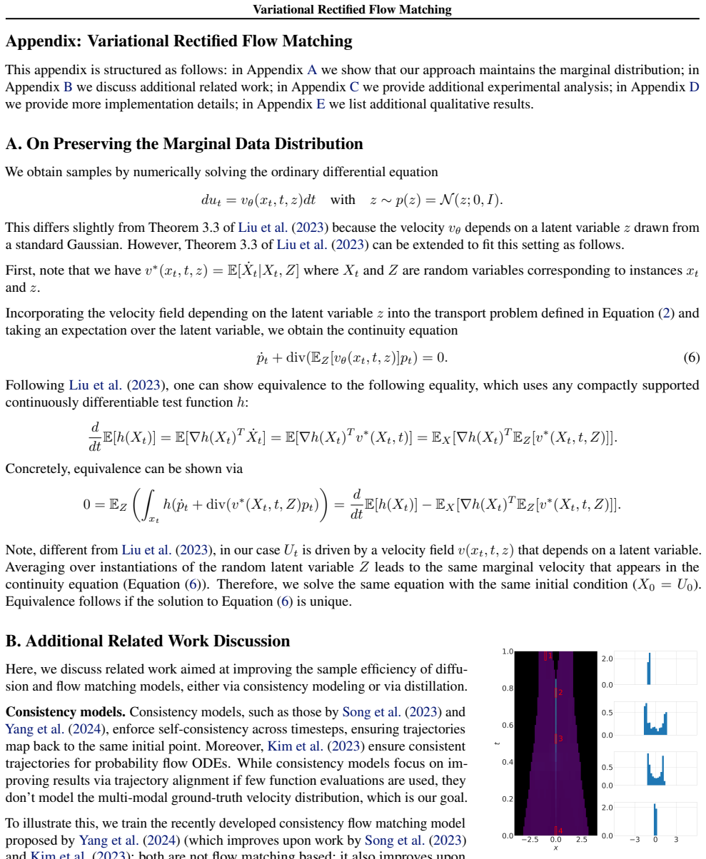
The central object is the latent-conditioned velocity field vθ(xt, t, z), trained with the variational objective E[−Ez∼qφ ||vθ(xt, t, z) − (x1 − x0)||² − DKL(qφ|p(z))]. The latent z is the mechanism that disambiguates crossing ground-truth velocities at the same (xt, t), turning the velocity model into a Gaussian mixture at each data-time location. At inference, sampling z once from the prior before ODE integration selects a flow direction for the whole trajectory.
What would settle it
On the paper's synthetic 1D bimodal example, estimate both sides of d/dt E[h(xt)] = E[∇h(xt)^T E_z[vθ(xt, t, z)]] for a compactly supported smooth test function h using the trained model; if the difference exceeds numerical solver tolerance, the marginal-preservation guarantee in Appendix A fails.
Extended reading notes
Core claim
The central claim is that the velocity field in rectified flow matching should be modeled as a Gaussian mixture rather than a single deterministic function. Because training couples each source sample to a random target sample, the ground-truth velocity v = x1 - x0 at an interpolated point xt = (1-t)x0 + tx1 points in multiple directions; an L2 regression learns the conditional expectation and averages them away. The paper's variational rectified flow matching instead learns a latent-conditioned velocity vθ(xt, t, z) with a recognition model qφ(z|x0, x1, xt, t) at training and a standard Gaussian prior at inference. The resulting objective replaces the single-Gaussian log-likelihood of the empirical velocity with an ELBO over z, differing from classic rectified flow only by one latent sampling step during training. The authors claim this preserves the marginal data distribution (by extending the rectified flow theorem to latent-conditioned velocities), captures multi-modal flow directions, and improves generation quality and controllability.
Load-bearing premise
The proof that the learned ODE preserves the target distribution assumes the latent variable z is independent of the state xt at each time, even though xt is produced by an ODE driven by z; the training objective does not guarantee this independence.
Editorial extensions
If this is right
- If the central claim holds, flow-matching models no longer need to sacrifice multi-modality when using random source-target couplings; the latent keeps ambiguous directions and produces straighter, crossable trajectories at the same training budget.
- On ImageNet 256x256, the paper's V-SiT-XL improves FID-50K from 17.2 to 14.6 at 400K steps and from 13.1 to 10.6 at 800K steps without classifier-free guidance, and from 5.40 to 4.91 with guidance at 400K steps.
- The latent variable becomes a controllable axis: in MNIST experiments a 2D latent smoothly interpolates between digit styles, and in CIFAR-10 it controls color and content without extra conditioning signals.
- Training cost is close to classic rectified flow: one extra posterior forward/backward pass, and inference adds only a single sample from the prior before ODE integration.
- The variational formulation is orthogonal to consistency-model and distillation approaches, so the paper suggests combining it with those acceleration techniques as a natural next step.
Reading between the lines
- The strongest empirical gains do not by themselves settle the theoretical question: if the latent z and the state xt are dependent, the Appendix A marginal-preservation argument is incomplete, and the improvements could come from an easier optimization landscape or an implicit regularizer rather than exact marginal transport.
- A direct mechanism check would be to measure the conditional variance of vθ(xt, t, z) at fixed (xt, t); the method should show nonzero variance matching the ground-truth ambiguity, whereas classic rectified flow collapses it.
- The controllability result suggests a practical extension: if the latent is trained with attribute labels, it could become a general-purpose style or class knob for flow-matching models, going beyond the 2D MNIST interpolation demonstrated in the paper.
Editorial analysis
A structured set of objections, weighed in public.
Referee Report
Summary. The paper proposes Variational Rectified Flow Matching (V-RFM), which augments rectified flow matching with a latent variable z that conditions the learned velocity field. The motivation is that classic rectified flow matching regresses ground-truth velocities that are multi-modal at the same data-time location, and the mean-squared-error loss averages them into a uni-modal, curved field. The authors introduce a variational objective that lower-bounds the log-likelihood of the empirical velocity and trains a posterior q_phi(z|x0,x1,xt,t) with a KL penalty, while at inference z is sampled from the prior and a single ODE trajectory is integrated. Experiments on synthetic 1D/2D data, MNIST, CIFAR-10, and ImageNet 256x256 show consistent FID improvements, especially at low numbers of function evaluations, and qualitative evidence that the latent provides controllability. Appendix A claims a theoretical guarantee that the learned ODE preserves the marginal data distribution, extending Theorem 3.3 of Liu et al. (2023).
Significance. If the empirical results hold, the paper makes a useful contribution: it directly targets the ambiguity in rectified flow matching and shows consistent gains across scales, including a 2.6-point FID improvement over SiT-XL on ImageNet at 400K steps (Table 2). The synthetic 1D experiments provide interpretable evidence that the learned velocity distribution captures the true bi-modality, which is a compelling demonstration. The paper also introduces a clean variational interpretation of flow matching. However, the central theoretical claim in Appendix A is not established as written: the proof that the learned ODE preserves the target marginal contains a gap that is load-bearing. The empirical contribution may stand independently, but the paper's stated theoretical guarantee needs correction or removal.
major comments (2)
- [Appendix A, Eq. (6) and following derivation] The marginal-preservation proof is incorrect as written. The inference ODE dX_t = v_theta(X_t,t,Z) dt with Z sampled once from p(z) induces a joint distribution over (X_t,Z) in which X_t and Z are dependent for t>0 whenever v_theta depends on Z. The continuity equation for the marginal p_t(x) is therefore not Eq. (6): averaging the per-latent continuity equation over z gives div(E_Z[v_theta(x,t,Z) p_t(x|Z)]), not div(E_Z[v_theta(x,t,Z)] p_t(x)). The subsequent equality E[∇h(X_t)^T v*(X_t,t)] = E_X[∇h(X_t)^T E_Z[v*(X_t,t,Z)]] would require X_t to be independent of Z, which is not implied by the variational objective (5) and generically fails. Thus the proof does not establish marginal preservation, and the claimed extension of Theorem 3.3 of Liu et al. (2023) is not proven. The authors should either provide a correct argument (e.g., by modifying inference to resample z at each step, or by showing a conditional-independence property that the objective enforces), or explicitly remove or qualify this theoretical claim.
- [Section 3.1, derivation of Eq. (5)] The variational lower bound in Eq. (5) is derived for a single empirical velocity v = x1 - x0, but the recognition model q_phi is conditioned on x0, x1, xt, and t. At inference, z is drawn from the prior N(0,I), whereas training samples z from q_phi. The standard VAE argument assumes the aggregate posterior roughly matches the prior; however, with the small KL weights used in several experiments (e.g., 2e-3 on ImageNet), this match is not guaranteed. This may explain part of the controllability results, but it also means the training objective does not explicitly enforce that the prior over z corresponds to meaningful semantic modes. This is not a fatal flaw, but it should be discussed as a limitation, especially because the claimed theoretical guarantee would require a stronger relationship between the training and inference latents.
minor comments (5)
- [Section 3.1, Eq. (3)] The notation p(x1 - x0|xt,t) is confusing, as x1 - x0 is a velocity vector rather than a random variable that one typically denotes in a probability density; clarifying that this is the density of the empirical velocity would improve readability.
- [Section 4.5] The phrase 'we use the Euler-Maruyama sampler with the SDE solver' is unclear because the paper otherwise describes deterministic ODE integration; specify whether this is a stochastic differential equation with injected noise or a deterministic ODE solver.
- [Table 1 caption] The final column is labeled 'Adaptive' but the caption does not define it; it should state that this refers to the adaptive-step Dopri5 solver.
- [Appendix D.1] The link in the footnote 'https://github.com/YangLing0818/consistency flow matching' contains a space and is not a valid URL; it should be corrected or removed.
- [Figure 2] The axis labels are small and the legends are not clearly visible; enlarging the fonts would help readers compare the metrics.
Circularity Check
Appendix A's marginal-preservation proof assumes the prior-averaged velocity is the marginal velocity, which is the very conclusion it claims to establish.
-
self definitional
[Appendix A, around Eq. (6) and the test-function display]
"First, note that we have v∗(xt, t, z) = E[ ˙Xt|Xt, Z] ... Incorporating the velocity field depending on the latent variable z into the transport problem defined in Equation (2) and taking an expectation over the latent variable, we obtain the continuity equation ˙pt + div(EZ[vθ(xt, t, z)]pt) = 0. (6) ... Averaging over instantiations of the random latent variable Z leads to the same marginal velocity that appears in the continuity equation (Equation (6)). Therefore, we solve the same equation with the same initial condition ( X0 = U0)."
Eq. (6) posits the continuity equation with the prior-marginal velocity E_Z[vθ(xt,t,z)]. The proof's task is to show that the ODE dXt = vθ(Xt,t,Z)dt with a single latent draw has exactly this marginal dynamics. Instead, the paper asserts this twice: 'taking an expectation over the latent variable, we obtain the continuity equation' and 'Averaging over instantiations ... leads to the same marginal velocity.' Because Z is drawn once and then held fixed, Xt and Z are dependent for t>0; the marginal velocity is E[vθ(Xt,t,Z)|Xt], not the unconditional average E_Z[vθ(xt,t,z)]. The displayed identity E[∇h(Xt)^T v*(Xt,t)] = EX[∇h(Xt)^T E_Z[v*(Xt,t,Z)]] is precisely the conditional-vs-marginal equality that needs proof.
full rationale
The empirical contribution—variational rectified flow matching with a latent variable, trained by the variational lower bound in Eq. (5)—is self-contained and not circular. The derivation of Claim 1 is a legitimate Gaussian-transport calculation, and the objective derivation from a conditional Gaussian velocity model to the MSE loss is standard. The circularity is confined to the theoretical marginal-preservation claim in Appendix A. There the paper intends to extend Liu et al. (2023) Theorem 3.3 to a latent-dependent velocity field, but the proof defines the continuity equation with the prior-average velocity E_Z[vθ] and then asserts that averaging over the latent 'leads to the same marginal velocity' and hence 'we solve the same equation.' That is the target statement. No load-bearing self-citation is involved; the only same-author citation (Zhang et al., 2025) is a concurrent-work comparison and does not support any derivation. Because the central theoretical guarantee is thus supported by an assumption that is equivalent to the conclusion, while the empirical FID results remain independent, the appropriate score is 6 (partial circularity).
Assumptions & free parameters
free parameters (2)
- KL divergence loss weight =
1.0 (1D), 0.1 (2D), 1e-3 (MNIST), 2e-3/5e-3 (CIFAR-10), 2e-3 (ImageNet)
- Latent variable dimension =
4 (1D), 8 (2D), 2 (MNIST), 768 (CIFAR-10), 1152 (ImageNet)
assumptions (4)
- domain assumption The conditional velocity distribution p(v|xt,t,z) is Gaussian with identity covariance
- domain assumption The continuity equation (6) has a unique solution in the relevant function space
- ad hoc to paper Z is independent of Xt when marginalizing the velocity field in the proof
- domain assumption The source distribution p0 is known and the velocity field is regular enough for ODE integration
invented entities (1)
-
Latent variable z (multi-modal direction selector)
independent evidence
Cite this review
Pith. "Pith review of Variational Rectified Flow Matching." pith.science (2026). https://pith.science/paper/RYKZRJN6
@misc{pith2026250209616,
  author       = {Pith},
  title        = {Pith review of: Variational Rectified Flow Matching},
  year         = {2026},
  howpublished = {\url{https://pith.science/paper/RYKZRJN6}},
  note         = {Machine review of arXiv:2502.09616}
}
read the original abstract
We study Variational Rectified Flow Matching, a framework that enhances classic rectified flow matching by modeling multi-modal velocity vector-fields. At inference time, classic rectified flow matching 'moves' samples from a source distribution to the target distribution by solving an ordinary differential equation via integration along a velocity vector-field. At training time, the velocity vector-field is learnt by linearly interpolating between coupled samples one drawn from the source and one drawn from the target distribution randomly. This leads to ''ground-truth'' velocity vector-fields that point in different directions at the same location, i.e., the velocity vector-fields are multi-modal/ambiguous. However, since training uses a standard mean-squared-error loss, the learnt velocity vector-field averages ''ground-truth'' directions and isn't multi-modal. In contrast, variational rectified flow matching learns and samples from multi-modal flow directions. We show on synthetic data, MNIST, CIFAR-10, and ImageNet that variational rectified flow matching leads to compelling results.
Figures


Figures from the paper (12 more)




Forward citations
Cited by 2 Pith papers
-
Source-Lifted Flow Matching for Intervenable Multimodal Imitation
Orthogonal Source Lifting makes flow-matching imitation intervenable by selecting only the source endpoint, changing future routes in 91.1% of matched-prefix tests while keeping free-deployment performance strong.
-
Hierarchical Rectified Flow Matching with Mini-Batch Couplings
Mini-batch couplings in data and velocity space simplify the hierarchy of velocity distributions in hierarchical rectified flow matching, improving low-step generation quality.
Reference graph
Works this paper leans on
-
[3]
These results demonstrate that V-RFM outperforms the consistency flow matching baseline across various evaluation steps for synthetic data, with V-RFM showing superior performance when the number of evaluation steps exceeds 2 for MNIST and 5 for CIFAR-10. Importantly, while consistency flow matching achieves strong performance for a low number of evaluati...
-
[4]
Understanding diffusion models: A unified perspec- tive
Luo, C. Understanding diffusion models: A unified perspec- tive. In arXiv preprint arXiv:2208.11970,
-
[6]
Dif- fuseV AE: Efficient, controllable and high-fidelity gener- ation from low-dimensional latents
Pandey, K., Mukherjee, A., Rai, P., and Kumar, A. Dif- fuseV AE: Efficient, controllable and high-fidelity gener- ation from low-dimensional latents. In arXiv preprint arXiv:2201.00308,
-
[7]
Yan, H., Liu, X., Pan, J., Liew, J. H., Liu, Q., and Feng, J. Perflow: Piecewise rectified flow as universal plug- and-play accelerator. arXiv preprint arXiv:2405.07510,
-
[8]
Consistency flow matching: Defining straight flows with velocity consis- tency
Yang, L., Zhang, Z., Zhang, Z., Liu, X., Xu, M., Zhang, W., Meng, C., Ermon, S., and Cui, B. Consistency flow matching: Defining straight flows with velocity consis- tency. arXiv preprint arXiv:2407.02398,
-
[9]
As expected, we observe that classic consistency modeling does not capture the multi-modal velocity distribution, unlike the proposed V-RFM. 1https://github.com/YangLing0818/consistency flow matching 11 Variational Rectified Flow Matching 2 5 8 10 16 20 Evaluation Steps 4 3 2 1 0 True Log-Likelihood Rectified FM Consistency FM VRFM (Ours) 2 5 8 10 16 20 E...
work page 2024
-
[10]
(6) Following Liu et al. (2023), one can show equivalence to the following equality, which uses any compactly supported continuously differentiable test function h: d dt E[h(Xt)] = E[∇h(Xt)T ˙Xt] = E[∇h(Xt)T v∗(Xt, t)] = EX [∇h(Xt)T EZ[v∗(Xt, t, Z)]]. Concretely, equivalence can be shown via 0 = EZ Z xt h( ˙pt + div(v∗(Xt, t, Z)pt) = d dt E[h(Xt)] − EX [∇...
work page 2023
-
[13]
36.5M 166.655 36.188 14.396 5.557 4.640 3.822 3.655 I-CFM (Liu et al., 2023; Tong et al.,
work page 2023
Show all 18 references
-
[16]
Higher scores indicate better performance
2.786 7.143 8.326 8.770 8.872 9.022 9.041 1 V-RFM (adaptive norm, x1, 2e-3) 3.943 7.728 8.499 8.973 9.050 9.168 9.171 2 V-RFM (adaptive norm, x1, 5e-3) 3.083 7.202 8.342 8.868 8.997 9.166 9.183 3 V-RFM (adaptive norm, x1 + t, 5e-3) 4.460 7.930 8.583 9.007 9.104 9.220 9.238 3 V...
2023
-
[17]
166.655 36.188 14.396 5.557 4.640 3.822 3.655 I-CFM (Liu et al., 2023; Tong et al.,
2023
-
[64]
The training batch size is 1000, and we employ the standard rectified flow objective, i.e., we compute the current data via xt = (1 − t)x0 + tx1, the ground truth velocity via v(x0, x1, t) = x1 − x0, and we use the L2 loss for supervision. For consistency flow matching, we ado...
2024
-
[128]
The decoder maintains the same structure as the baseline, with the first MLP layer adjusted to accommodate the increased channel input
The conditional latent embedding z is concatenated with the embeddings for time t and data x. The decoder maintains the same structure as the baseline, with the first MLP layer adjusted to accommodate the increased channel input. For the posterior model qϕ, we employ a similar...
2023
-
[256]
The KL loss weight is set to 2 × 10⁻³, and the posterior model qϕ takes x1 as input. To ensure a fair comparison, we strictly adhere to the original training recipe of SiT (Ma et al., 2024), i.e., we don’t tune learning rate, decay or warm-up schedules, AdamW parameters, or em...
2024
-
[2018]
Variational Flow Matching for Graph Generation
Eijkelboom, F., Bartosh, G., Naesseth, C., Welling, M., and van de Meent, J.-W. Variational Flow Matching for Graph Generation. In arXiv preprint arXiv:2406.04843,
-
[2022]
SiT: Exploring Flow and Diffusion-based Generative Models with Scalable Inter- polant Transformers
Ma, N., Goldstein, M., Albergo, M., Boffi, N., Vanden- Eijnden, E., and Xie, S. SiT: Exploring Flow and Diffusion-based Generative Models with Scalable Inter- polant Transformers. In arXiv preprint arXiv:2401.08740,
-
[2023]
Stochastic Interpolants: A unifying framework for flows and diffu- sions
Albergo, M., Boffi, N., and Vanden-Eijnden, E. Stochastic Interpolants: A unifying framework for flows and diffu- sions. In arXiv preprint arXiv:2303.08797,
-
[2024]
Deep Residual Learning for Image Recognition
He, K., Zhang, X., Ren, S., and Sun, J. Deep Residual Learning for Image Recognition. In https://arxiv.org/abs/1512.03385,
-
[2025]
10 Variational Rectified Flow Matching Appendix: Variational Rectified Flow Matching This appendix is structured as follows: in Appendix A we show that our approach maintains the marginal distribution; in Appendix B we discuss additional related work; in Appendix C we provide ...
2023
Reviewed August 7, 2026 · model on record in the stance chip above.
Discussion (0). Sign in to comment.