Quantum fluctuation energies over a spatially inhomogeneous field background in a chiral soliton model
Pith reviewed 2026-05-23 01:37 UTC · model grok-4.3
The pith
Finite quantum fluctuation energies of quarks over a chiral soliton background are evaluated numerically after renormalization by Born subtraction of phase shifts.
A machine-rendered reading of the paper's core claim, the machinery that carries it, and where it could break.
Core claim
The effective Hamiltonian for quarks in the static spherical hedgehog background is diagonalized by parity and grand spin; the resulting phase shifts determine the density of states, which after Born subtraction and diagram compensation yields finite numerical values for the fluctuation energy in each channel.
What carries the argument
Born-subtracted phase-shift density of states used to evaluate the renormalized one-loop sum over the Dirac spectrum.
If this is right
- The total classical plus quantum energy of the soliton receives well-defined additive contributions from each parity-grand-spin sector.
- Stability or binding-energy estimates for the soliton can be refined by including these channel-by-channel corrections.
- The same renormalization procedure applies directly to other static background configurations that admit a phase-shift analysis.
Where Pith is reading between the lines
- Extending the calculation to non-spherical or time-dependent backgrounds would test whether the finite remainder remains well-defined.
- Comparing the channel contributions to observed baryon mass splittings could constrain the parameters of the underlying chiral model.
- The method supplies a concrete benchmark for other regularization schemes that aim to compute the same one-loop correction.
Load-bearing premise
Subtracting the Born approximation to the phase shift together with compensating Feynman diagrams isolates a physically meaningful finite remainder that does not depend on the ultraviolet cutoff.
What would settle it
A numerical result in which the renormalized energy still changes when the momentum cutoff is increased or when more partial waves are included would show that the finite remainder has not been isolated.
Figures
read the original abstract
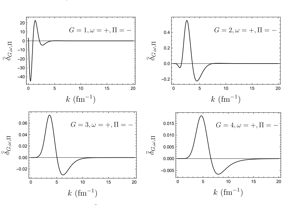
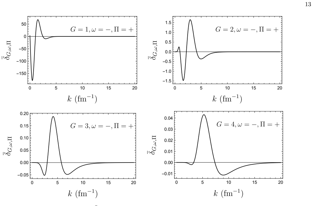
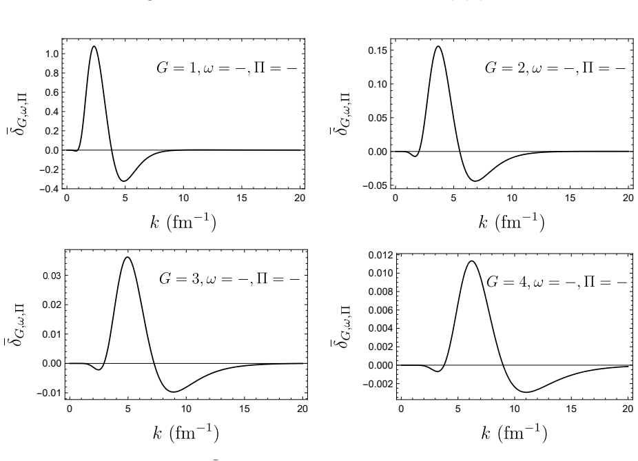
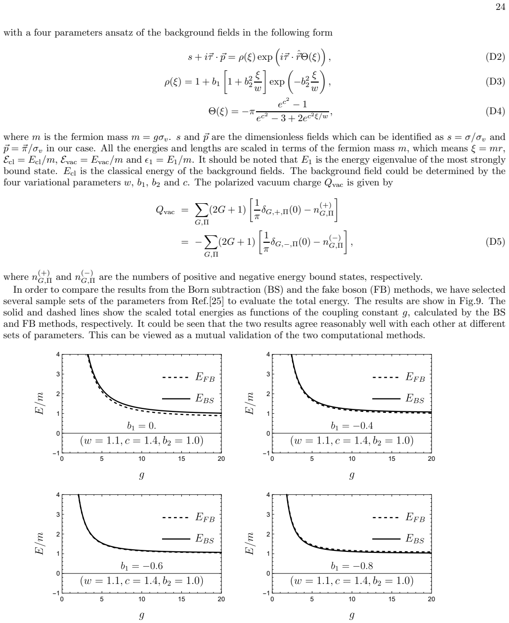
Based on chiral soliton models, the quantum fluctuation energies of quarks over a spatially inhomogeneous meson field background have been thoroughly studied. We have used a systematic calculation scheme initiated by Schwinger, in which the loop quantum fluctuation energies are evaluated by a nontrivial level summation over the eigenvalue spectrum of the effective Hamiltonian of the system. The effective Hamiltonian can be constructed by one loop effective action of fluctuations of quarks over a static chiral soliton field background. The corresponding Dirac equation is obtained. In a static and spatially spherical case and by the hedgehog ansatz the radial part and the angular part of the grand spin of the wave function for the Dirac equation can be separated. Due to the soliton background the eigenvalue spectrum are distorted. The scattering phase shift can be determined by solve the radial equations at different momentum. The density of states in momentum space can be derived. The effective Hamiltonian has been diagonalized in a Hilbert space where the eigenfunctions are labeled by the parity, grand spin and energy. The renormalization scheme can be carried out by a Born subtraction of the phase shift and the compensating Feynman diagram renormalization. Finally the finite quantum fluctuation energies over chiral soliton background at different parities and grand spins have been numerically evaluated, compared and discussed.
Editorial analysis
A structured set of objections, weighed in public.
Referee Report
Summary. The manuscript computes quantum fluctuation energies of quarks over a static chiral soliton background in a chiral soliton model. It constructs the one-loop effective action, derives the Dirac equation under the hedgehog ansatz, separates variables by parity and grand spin, extracts scattering phase shifts from the radial equations, applies Born subtraction plus compensating Feynman diagrams for renormalization, and reports numerical values for the finite per-channel energies.
Significance. If the subtracted phase-shift sums plus counterterms can be shown to produce cutoff-independent results, the channel-by-channel numerical values would supply concrete data on quantum corrections in inhomogeneous meson backgrounds, useful for refining soliton-model predictions of baryon properties. The work follows a standard Schwinger proper-time/level-density approach but currently lacks the convergence diagnostics needed to certify the output.
major comments (1)
- [Renormalization and numerical evaluation] Renormalization procedure (described after the phase-shift extraction): the central claim that Born subtraction of the phase shift together with compensating Feynman diagrams isolates a finite, physically meaningful remainder requires explicit numerical verification that the per-channel energies are stable when the momentum cutoff or basis size is varied and that the leading UV divergence cancels. No such stability tests or cancellation plots are reported, leaving the finiteness of the quoted energies unsubstantiated.
minor comments (2)
- [Abstract] The abstract states that the energies 'have been numerically evaluated' but supplies neither error estimates, convergence tables, nor comparisons with independent regularization schemes.
- [Methods] Notation for the grand-spin channels and the precise definition of the subtracted phase-shift integral should be stated explicitly before the numerical results are presented.
Simulated Author's Rebuttal
We thank the referee for the careful reading of our manuscript on quantum fluctuation energies over chiral soliton backgrounds. The single major comment concerning explicit numerical verification of renormalization stability is addressed point-by-point below. We will strengthen the presentation accordingly.
read point-by-point responses
-
Referee: [Renormalization and numerical evaluation] Renormalization procedure (described after the phase-shift extraction): the central claim that Born subtraction of the phase shift together with compensating Feynman diagrams isolates a finite, physically meaningful remainder requires explicit numerical verification that the per-channel energies are stable when the momentum cutoff or basis size is varied and that the leading UV divergence cancels. No such stability tests or cancellation plots are reported, leaving the finiteness of the quoted energies unsubstantiated.
Authors: We agree that explicit numerical checks would strengthen the manuscript. The Born subtraction plus compensating Feynman diagrams is constructed to cancel the leading UV divergence analytically, as is standard in phase-shift renormalization of Dirac spectra in soliton backgrounds; the quoted per-channel values are the resulting finite remainders. To provide direct evidence of stability, the revised version will add plots of selected per-channel energies versus momentum cutoff (and, where applicable, basis size), demonstrating convergence to cutoff-independent plateaus beyond a threshold value. A brief discussion of these diagnostics will be inserted after the description of the renormalization scheme. revision: yes
Circularity Check
No circularity; direct numerical evaluation of renormalized spectrum
full rationale
The derivation proceeds by constructing the Dirac Hamiltonian from the one-loop effective action in the hedgehog background, separating variables in grand spin and parity, extracting phase shifts from the radial scattering solutions, performing the standard Born subtraction plus compensating diagrams, and summing the resulting finite level-shift contribution. None of these steps defines the output energies in terms of themselves or renames a fitted quantity as a prediction; the renormalization procedure is an external subtraction scheme applied to the computed spectrum, and the final per-channel energies are obtained by direct summation rather than by construction from input parameters. No self-citation is invoked as a load-bearing uniqueness theorem.
Axiom & Free-Parameter Ledger
axioms (2)
- domain assumption The hedgehog ansatz correctly captures the static spherical soliton background and allows separation of radial and angular variables.
- domain assumption The Born subtraction plus Feynman-diagram counterterms remove all ultraviolet divergences while leaving a finite physical remainder.
Reference graph
Works this paper leans on
-
[1]
School of Physics, Hubei University, Wuhan, Hubei 430062 , China and
-
[2]
Key Laboratory of Quark and Lepton Physics (MOE) and Insti tute of Particle Physics, Central China Normal University, Wuhan, Hubei 430079, Chin a Based on chiral soliton models, the quantum fluctuation ener gies of quarks over a spatially in- homogeneous meson field background have been thoroughly stu died. We have used a systematic calculation scheme initi...
work page internal anchor Pith review Pith/arXiv arXiv 2026
-
[3]
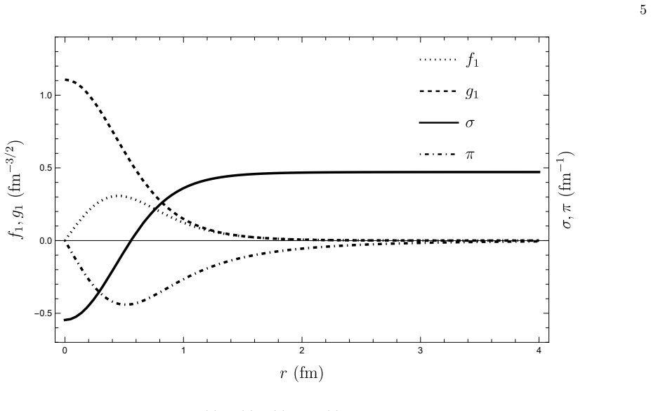
G = 0 case When G = 0, the equations of negative parity are { g′ 1 + 2 rg1 − (ε +gσ )f1 − gπg 1 = 0, f ′ 1 + (ε − gσ )g1 +gπf 1 = 0, (45) Atr → ∞ , considering σ (r) → σv, π → 0, the asymptotic forms of the equations (17) are { g′ 1 + 2 rg1 − (ε +gσv)f1 = 0, f ′ 1 + (ε − gσv)g1 = 0, (46) From the characteristics of the equations, combined with the recu rs...
-
[4]
G ̸= 0 case For the case of G ̸= 0 and the parity Π = − (− 1)G, the solution has a matrix form. Usually the first order differential equations should be decoupled to two sets of the second order equ ations of the upper part and the lower part of the Dirac spinor. Each part is still a two flavor isospinor. For the upper p art the radial wave functions are g1(...
-
[5]
gs order equations: v(1)(1, 0)′ 1 +v(1)(1, 0) 1 h′ G+1 hG+1 + G + 2 r v(1)(1, 0) 1 − (ε − gσv) hG hG+1 u(1)(1, 0) 1 +βσs = 0; v(1)(1, 0)′ 2 +v(1)(1, 0) 2 h′ G− 1 hG− 1 − G − 1 r v(1)(1, 0) 2 + (ε − gσv) hG hG− 1 u(1)(1, 0) 2 = 0; u(1)(1, 0)′ 1 +u(1)(1, 0) 1 h′ G hG − G ru(1)(1, 0) 1 + (ε +gσv)hG+1 hG v(1)(...
-
[6]
g2 s order equations: v(1)(2, 0)′ 1 +v(1)(2, 0) 1 h′ G+1 hG+1 + G + 2 r v(1)(2, 0) 1 − (ε − gσv) hG hG+1 u(1)(2, 0) 1 +σsu(1)(1, 0) 1 = 0; v(1)(2, 0)′ 2 +v(1)(2, 0) 2 h′ G− 1 hG− 1 − G − 1 r v(1)(2, 0) 2 + (ε − gσv) hG hG− 1 u(1)(2, 0) 2 − σsu(1)(1, 0) 2 = 0; u(1)(2, 0)′ 1 +u(1)(2, 0) 1 h′ G hG − G ru(1)(2...
-
[7]
gp order equations: v(1)(0, 1)′ 1 +v(1)(0, 1) 1 h′ G+1 hG+1 + G + 2 r v(1)(0, 1) 1 − (ε − gσv) hG hG+1 u(1)(0, 1) 1 + π 1 + 2G = 0; v(1)(0, 1)′ 2 +v(1)(0, 1) 2 h′ G− 1 hG− 1 − G − 1 r v(1)(0, 1) 2 + (ε − gσv) hG hG− 1 u(1)(0, 1) 2 + 2 √ G(1 +G)π 1 + 2G = 0; u(1)(0, 1)′ 1 +u(1)(0, 1) 1 h′ G hG − G ru(1)...
-
[8]
g2 p order equations: v(1)(0, 2)′ 1 +v(1)(0, 2) 1 h′ G+1 hG+1 + G + 2 r v(1)(0, 2) 1 − (ε − gσv) hG hG+1 u(1)(0, 2) 1 + π 1 + 2Gv(1)(0, 1) 1 − 2 √ G(1 +G)π 1 + 2G v(1)(0, 1) 2 = 0; v(1)(0, 2)′ 2 +v(1)(0, 2) 2 h′ G− 1 hG− 1 − G − 1 r v(1)(0, 2) 2 + (ε − gσv) hG hG− 1 u(1)(0, 2) 2 + π 1 + 2Gv(1)(0, 1) 2 ...
-
[9]
gsgp order equations: v(1)(1, 1)′ 1 +v(1)(1, 1) 1 h′ G+1 hG+1 + G + 2 r v(1)(1, 1) 1 − (ε − gσv) hG hG+1 u(1)(1, 1) 1 +σsu(1)(0, 1) 1 + π 1 + 2Gv(1)(1, 0) 1 − 2 √ G(1 +G)π 1 + 2G v(1)(1, 0) 2 = 0; v(1)(1, 1)′ 2 +v(1)(1, 1) 2 h′ G− 1 hG− 1 − G − 1 r v(1)(1, 1) 2 + (ε − gσv) hG hG− 1 u(1)(1, 1) 2 − σsu(1...
-
[10]
gs order equations: v(1)(1, 0)′′ 1 + 2 rv(1)(1, 0)′ 1 ( 1 + rh′ G+1 hG+1 ) + ( − σ ′ s εv )h′ G+1 hG+1 + ( − σ ′ s εv )G + 2 r = 0, v(1)(1, 0)′′ 2 + 2 rv(1)(1, 0) 2 ′ ( 1 + rh′ G+1 hG+1 ) + 2(2G + 1) r2 v(1)(1, 0) 2 = 0, (C5) v(2)(1, 0)′′ 1 + 2 rv(2)(1, 0)′ 1 ( 1 + rh′ G− 1 hG− 1 ) − 2(2G + 1) r2 v(2)(1,...
-
[11]
g2 s order equations: − σ ′ s εv ( v(1)(1, 0)′ 1 +v(1)(1, 0) 1 h′ G+1 hG+1 ) + ( − σ ′ s εv )G + 2 r v(1)(1, 0) 1 + σ ′ sσs ε2 v h′ G+1 hG+1 + σ ′ sσs ε2 v G + 2 r − (σ 2 s + 2σvσs) +v(1)(2, 0)′′ 1 + 2 rv(1)(2, 0)′ 1 ( 1 + rh′ G+1 hG+1 ) = 0, − σ ′ s εv ( v(1)(1, 0)′ 2 +v(1)(1, 0) 2...
-
[12]
gp order equations: v(1)(0, 1)′′ 1 + 2 rv(1)(0, 1)′ 1 ( 1 + rh′ G+1 hG+1 ) + G + 1 2G + 1 2 rπ − π ′ 2G + 1 = 0, v(1)(0, 1)′′ 2 + 2 rv(1)(0, 1)′ 2 ( 1 + rh′ G+1 hG+1 ) + 2(2G + 1) r2 v(1)(0, 1) 2 − π r 2 √ G(G + 1) 2G + 1 + 2 √ G(G + 1) 2G + 1 π ′ = 0, (C9) v(2)(0, 1)′′ 1 + 2 rv(2)(0, 1)′...
-
[13]
g2 p order equations: ( − π ′ 2G + 1 + 2 r G + 1 2G + 1π ) v(1)(0, 1) 1 + 2 √ G(G + 1) 2G + 1 ( π ′ − π r ) v(1)(0, 1) 2 − π 2 +v(1)(0, 2)′′ 1 + 2 rv(1)(0, 2)′ 1 ( 1 + rh′ G+1 hG+1 ) = 0, 2 √ G(G + 1) 2G + 1 ( π ′ − π r ) v(1)(0, 1) 1 + ( π ′ 2G + 1 + 2 r G 2G + 1π ) v(1)(0, 1) 2 +v(1)(0, 2)′′ 2 + 2 rv...
-
[14]
The above equations could be numerically solved order by order
gsgp order equations: ( − π ′ 2G + 1 + 2 r G + 1 2G + 1π ) v(1)(0, 1) 1 + 2 √ G(G + 1) 2G + 1 ( π ′ − π r ) v(1)(1, 0) 2 + σ ′ s εv π 2G + 1 − σ ′ s εv ( v(1)(0, 1)′ 1 +v(1)(0, 1) 1 h′ G+1 hG+1 ) − σ ′ s εv G + 2 r v(1)(0, 1) 1 +v(1)(1, 1)′′ 1 + 2...
-
[15]
M. N. Chernodub, Physical Review D 103, 054027 (2021)
work page 2021
-
[16]
Y. Chen, D. Li, and M. Huang, Physical Review D 106, 106002 (2022)
work page 2022
-
[17]
K. Fukushima and C. Sasaki, Progress in Particle and Nucl ear Physics 72, 99 (2013)
work page 2013
-
[18]
M. Buballa and S. Carignano, Progress in Particle and Nuc lear Physics 81, 39 (2015)
work page 2015
-
[19]
T. Brauner and N. Yamamoto, Journal of High Energy Physic s 2017, 1 (2017)
work page 2017
- [20]
-
[21]
J. Ishioka, Y. Liu, K. Shimatake, T. Kurosawa, K. Ichimur a, Y. Toda, M. Oda, and S. Tanda, Physical review letters 105, 176401 (2010)
work page 2010
-
[22]
N. Evans, K.-Y. Kim, M. Magou, Y. Seo, and S.-J. Sin, Journ al of High Energy Physics 2012, 1 (2012)
work page 2012
-
[23]
Voskresensky, Progress in Particle and Nuclear Physi cs 130, 104030 (2023)
D. Voskresensky, Progress in Particle and Nuclear Physi cs 130, 104030 (2023)
work page 2023
-
[24]
P. Lakaschus, M. Buballa, and D. H. Rischke, Phys. Rev. D 103, 034030 (2021)
work page 2021
-
[25]
G. Endr˝ odi, T. G. Kov´ acs, and G. Mark´ o, Phys. Rev. Lett. 127, 232002 (2021)
work page 2021
-
[26]
C. Y. Cardall, M. Prakash, and J. M. Lattimer, The Astrop hysical Journal 554, 322 (2001)
work page 2001
-
[27]
A. Tsokaros, M. Ruiz, S. L. Shapiro, and K. b. o. Ury¯ u, Ph ys. Rev. Lett. 128, 061101 (2022)
work page 2022
- [28]
-
[29]
E. J. Ferrer, W. Gyory, and V. de la Incera, Phys. Rev. D 109, 036023 (2024)
work page 2024
- [30]
-
[31]
I. W. Stewart and P. G. Blunden, Phys. Rev. D 55, 3742 (1997)
work page 1997
- [32]
-
[33]
M. Shifman, A. Vainshtein, and M. Voloshin, Phys. Rev. D 59, 045016 (1999)
work page 1999
-
[34]
G. V. Dunne, Physics Letters B 467, 238 (1999)
work page 1999
- [35]
- [36]
- [37]
- [38]
- [39]
- [40]
- [41]
-
[42]
Schwinger, Physical Review 94, 1362 (1954)
J. Schwinger, Physical Review 94, 1362 (1954)
work page 1954
-
[43]
t Hooft, Physical Review D 14, 3432 (1976)
G. t Hooft, Physical Review D 14, 3432 (1976)
work page 1976
-
[44]
Shu, SCIENCE CHINA Physics, Mechanics & Astronomy 60, 041021 (2017)
S. Shu, SCIENCE CHINA Physics, Mechanics & Astronomy 60, 041021 (2017)
work page 2017
-
[45]
S. Shu, X. Li, and J.-R. Li, Nuclear Physics A 1014, 122256 (2021)
work page 2021
-
[46]
X. Li, S. Shu, and J.-R. Li, Physical Review C 105, 045203 (2022)
work page 2022
-
[47]
M. C. Birse and M. K. Banerjee, Physics Letters B 136, 284 (1984)
work page 1984
-
[48]
D. Diakonov, V. Y. Petrov, and P. Pobylitsa, Nuclear Phy sics B 306, 809 (1988)
work page 1988
-
[49]
C. V. Christov, A. Blotz, H.-C. Kim, P. Pobylitsa, T. Wat abe, T. Meissner, E. R. Arriola, and K. Goeke, Progress in Particle and Nuclear Physics 37, 91 (1996)
work page 1996
-
[50]
A. M´ ocsy, I. N. Mishustin, and P. J. Ellis, Phys. Rev. C 70, 015204 (2004)
work page 2004
-
[51]
P. Weng, B. Li, Y. Lyu, S. Shu, and H. Zhang, Physics Lette rs B 867, 139587 (2025)
work page 2025
-
[52]
Ma, Journal of Mathematical Physics 26, 1995 (1985)
Z. Ma, Journal of Mathematical Physics 26, 1995 (1985)
work page 1995
discussion (0)
Sign in with ORCID, Apple, or X to comment. Anyone can read and Pith papers without signing in.