REVIEW 3 major objections 5 minor 47 references
TimeCapsule: Solving the Jigsaw Puzzle of Long-Term Time Series Forecasting with Compressed Predictive Representations
T0 review · 3 major / 5 minor · reviewed 2026-08-16 · deepseek-v4-flash
Pith's one-line read TimeCapsule claims long-term multivariate forecasting reduces to one compression principle—shrink a 3D time-variate-level tensor, predict in the latent space, expand back—and reports best or near-best error on ten benchmarks.
desk verdict TimeCapsule is a well-built, honestly ablated architecture, but its SOTA claim is not established because the baselines ran with shorter tuned lookbacks while TimeCapsule used a fixed 512. read the letter →
The pith
A machine-rendered reading of the paper's core claim, the machinery that carries it, and where it could break.
The reading
What carries the argument
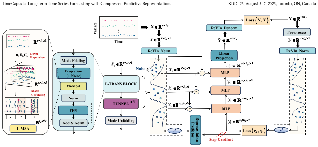
The load-bearing object is the 3D tensor representation of the series together with the mode product: a learned matrix multiplication along one axis of a tensor after folding the other two axes, used here to compress each dimension before attention is applied. TimeCapsule's Mode-Specific Multi-head Self-Attention (MoMSA) applies vanilla self-attention to the folded matrix in the compressed space, so the attention map is itself compressed; the transform is written as the product of an expanding and a compressing matrix, allowing lossy low-rank compression rather than fixed patching. The second mechanism is residual information back: each compression step records what was lost and concatenates it into the decoder, so the final forecast is not forced to recover everything from the capsule. The third is the JEPA internal forecast, which predicts the compressed representation of the future from the compressed representation of the past, using a stop-gradient EMA target encoder to supervise the latent space.
What would settle it
Rerun every baseline and TimeCapsule under identical preprocessing and hyperparameter search, with lookback fixed at 512 for all of them rather than searched for baselines alone, and also with each model given its own best lookback; if the reported margins vanish or reverse under either protocol, the central claim of universal superiority fails.
Extended reading notes
Core claim
The central claim is that long-term multivariate forecasting is best organised as a compression problem, not an architecture-design problem. TimeCapsule encodes an observed window $X \in \mathbb{R}^{v \times t_x \times 1}$ by sequentially compressing the temporal, level, and variate axes with learnable mode-product transforms, producing a small capsule $X_3 \in \mathbb{R}^{v_c \times t_c \times l}$. A single linear layer predicts the future capsule, and three MLP blocks expand it back to the real time axis, using stored residuals $B_1, B_2, B_3$ to return detail lost in compression. A Joint-Embedding Predictive Architecture loss compares the encoded observed representation with an EMA-encoded target representation and is added to the forecast loss. In the reported experiments, the model matches or approaches the best result across all datasets and horizons, and removing the residual feedback degrades performance sharply.
Load-bearing premise
The headline comparison assumes that giving TimeCapsule a fixed 512-step lookback while letting each baseline search its own lookback is a fair protocol; if the baselines were handicapped by suboptimal windows, the reported margins could shrink or reverse.
Editorial extensions
If this is right
- A single architecture with a weak transformer encoder and an MLP decoder can cover both datasets that need explicit multi-scale modelling and datasets where a pure MLP is nearly enough, by learning how much to compress rather than hard-coding patches.
- Long lookbacks become cheap: because the temporal axis is compressed before self-attention, a 512-step history can be processed without quadratic attention cost, and the paper's lookback study shows accuracy keeps improving as the window grows.
- The residual feedback is load-bearing: ablation shows that removing it causes a dramatic drop in accuracy, so any compressed-forecasting design must solve the information-recovery problem, not just the compression problem.
- The JEPA loss is a monitoring signal as much as a training signal: it decreases even without backpropagation, and including it in training helps on some datasets while being neutral on others, suggesting latent-space prediction can guide convergence.
Reading between the lines
- If the learned level-expansion matrix really decomposes the series into additive level components—the paper shows the sum of sub-level series nearly reconstructs the input—the same transform could be reused as a trainable, dataset-specific decomposition tool for other tasks, independent of forecasting.
- The comparison protocol deserves a direct stress test: rerun every baseline under the same fixed lookback of 512, and also rerun TimeCapsule under each baseline's searched lookback, to separate the benefit of the architecture from the benefit of the longer window.
- The JEPA target construction (zero-padding short targets, EMA-averaging long targets) is one design choice among several; comparing it against alternatives such as random chunk pooling or a learned target encoder would show whether the decreasing JEPA loss is a meaningful signal or a side effect of preprocessing.
Signed reviews
Editorial analysis
A structured set of objections, weighed in public.
Referee Report
Summary. The paper proposes TimeCapsule, a multivariate long-term time series forecasting architecture that treats the input as a 3D tensor with time, variate, and level dimensions. The encoder applies mode-specific multi-head self-attention with low-rank compression transforms (MoMSA) along each dimension, and residual information is passed back to a simple MLP decoder that reconstructs the future. A Joint-Embedding Predictive Architecture (JEPA) loss, computed between the compressed representation of the input and an EMA-encoded preprocessing of the target, is added as an auxiliary objective. Experiments on ten benchmarks compare TimeCapsule with eight TFB-derived baselines and report best or near-best MSE/MAE in most settings, together with ablations for residual compensation, compression dimensions, noise, block order, positional encoding, and a classification extension.
Significance. If the empirical claims hold, TimeCapsule is a useful contribution. It unifies multi-level modeling, multi-mode dependency capture, and linear projection in a relatively simple architecture, and it demonstrates how a JEPA-style loss can be attached to a forecasting model. The paper is candid about the auxiliary and dataset-dependent effect of the JEPA term, it ships code, and it provides component-level ablations and visualizations of learned transform matrices. The main risk is not internal circularity but external validity: the headline state-of-the-art claim rests on an asymmetric lookback protocol and on single-run baseline numbers, and several margins are smaller than the model's own seed-to-seed variability reported in the appendix.
major comments (3)
- [§5.1.2 / Table 1 caption / Appendix C.1] The headline comparison is asymmetric: TimeCapsule is evaluated with a fixed lookback of 512 for all datasets except ILI, while every baseline uses lookback lengths searched for the best performance. The caption does not report the actual lookbacks selected for the baselines; if those are shorter than 512, Table 1 conflates the architecture with access to a longer input context. Appendix C.1 (Fig. 8) shows that TimeCapsule's error consistently decreases as the lookback grows from 96 to 720 for ETTh1, Weather, PEMS04, and Traffic. Since many margins are tiny (e.g., Weather 96 MSE is 0.141 vs. 0.142 for the two TimeCapsule columns), a single lookback choice could reverse several rankings. Please re-run the baselines at T=512 under the TFB protocol, or run TimeCapsule at each baseline's searched lookback, and report both configurations side by side.
- [§4.2.3, Eq. (16)] The target preprocessing for the JEPA loss is a heuristic that is neither derived nor validated. Zero-padding when t_y < t_x and EMA-averaging chunks when t_y > t_x produce a target tensor of length t_x, but no evidence is given that this target is a meaningful prediction target in the representation space; for t_y > t_x, the EMA mixes future points across chunks in a way that may not correspond to any actual input-like sequence. Moreover, the JEPA loss itself is never defined: the text gives 'Loss(Enc_x(X), sg(Enc_y(Y))' with no closing parenthesis and no specification of the distance used. Because the paper's own ablation in §5.2.2 shows the JEPA effect is small and dataset-dependent, this missing definition and missing validation matter. Please specify the loss explicitly and compare the proposed padding/EMA scheme with simpler alternatives, such as using the last t_x points of the target without preprocessing.
- [Appendix B / Table 5] The robustness analysis reports standard deviations only for TimeCapsule, and only for four datasets, while all baseline numbers in Table 1 are point values taken from TFB. Given margins at the third decimal place, this is insufficient to substantiate the claim in §5.1.3 that TimeCapsule 'consistently achieves or approaches the best performance.' For example, the Weather 96 entry 0.141 in Table 1 is within one standard deviation of the 0.143±0.001 reported in Table 5, so a second-run difference of 0.002 could change the ranking. Please provide baseline error bars or a sensitivity analysis, at least for the settings where TimeCapsule's margin over the second-best model is smaller than the variability of either method.
minor comments (5)
- [§3, Definition 1] The definitions of Fold and Unfold appear to be swapped relative to standard tensor terminology: unfolding maps a tensor to a matrix and folding maps a matrix back to a tensor. Please correct the terminology or state the convention explicitly to avoid confusion in Eqs. (11)–(15).
- [§3 and §4.1] The text uses both 'mode production' and 'mode product'; these should be unified to 'mode product' throughout.
- [Appendix C.1] The text states that the lookback window ranges from 96 to 512, but the horizontal axis of Fig. 8 goes to 720. Align the text and figure.
- [Table 1] The row labeled '1st Count' at the bottom of the table is not explained in the caption. Please specify whether it counts best MSE, best MAE, or best on either metric, and over which set of settings.
- [§5.1.2] The hyperparameter selection is reported only as ranges (batch size 32–128, learning rate 1e-4 to 2e-3). Please list the per-dataset selected values for reproducibility, since the appendix reports multiple seeds but the main table is for a single seed (2021).
Circularity Check
No significant circularity: TimeCapsule's reported gains are empirical benchmark results against external TFB baselines, not quantities derived by construction from fitted parameters or self-citations.
full rationale
TimeCapsule is an empirical architecture paper. Its chain of reasoning is architectural: a 3D tensor encoding, mode-product compression, residual information back, a JEPA auxiliary loss, and a supervised forecasting objective. No equation in the paper reduces the forecast to a fitted constant or to the paper's own inputs. The compression dimensions are hyperparameters chosen from a small grid and reported in ablations; they are not renamed predictions. The JEPA target uses an EMA of the input encoder, but the paper explicitly and candidly shows the JEPA effect is small and dataset-dependent (Section 5.2.2, Fig. 5), so it is not load-bearing. There are no self-citations by the authors: the cited works (RevIn, iTransformer, JEPA, TFB) are independent and external. The only notable concern is the asymmetric lookback protocol: TimeCapsule uses a fixed T=512 while baselines use searched lookbacks (Table 1 caption), and Appendix C.1 shows longer lookbacks improve TimeCapsule. That is a fairness/correctness concern about benchmark comparability, not a circularity: the reported numbers are not derived by construction from the baseline numbers, and no fitted parameter is relabeled as a prediction. Because no specific reduction from output to input can be exhibited, the appropriate score is 0.
Assumptions & free parameters
free parameters (3)
- compression dimensions per dataset (t_c, l_c, v_c) =
selected from {1,4,8,32}; default (4,8,4)
- JEPA loss weight =
not explicitly reported
- number of tunnel blocks =
0 to 2
assumptions (6)
- domain assumption Mode-k product with low-rank factors C_T E_T compresses a time series while preserving information needed for forecasting.
- domain assumption The level dimension, expanded by a learned linear map, serves as a multi-scale or decomposition basis.
- ad hoc to paper Zero-padding or EMA-splitting the target (Eq. 16) yields a target representation comparable to the input representation for the JEPA loss.
- domain assumption Reversible instance normalization does not alter the stationarity of the series.
- standard math Standard tensor algebra operations (folding, unfolding, mode products) are correctly defined and computed.
- domain assumption Benchmark data splits and baseline results from TFB are accurate and comparable.
invented entities (1)
-
Level dimension (L)
Cite this review
Pith. "Pith review of TimeCapsule: Solving the Jigsaw Puzzle of Long-Term Time Series Forecasting with Compressed Predictive Representations." pith.science (2026). https://pith.science/paper/OIFCACSF
@misc{pith2026250412721,
  author       = {Pith},
  title        = {Pith review of: TimeCapsule: Solving the Jigsaw Puzzle of Long-Term Time Series Forecasting with Compressed Predictive Representations},
  year         = {2026},
  howpublished = {\url{https://pith.science/paper/OIFCACSF}},
  note         = {Machine review of arXiv:2504.12721}
}
read the original abstract
Recent deep learning models for Long-term Time Series Forecasting (LTSF) often emphasize complex, handcrafted designs, while simpler architectures like linear models or MLPs have often outperformed these intricate solutions. In this paper, we revisit and organize the core ideas behind several key techniques, such as redundancy reduction and multi-scale modeling, which are frequently employed in advanced LTSF models. Our goal is to streamline these ideas for more efficient deep learning utilization. To this end, we introduce TimeCapsule, a model built around the principle of high-dimensional information compression that unifies these techniques in a generalized yet simplified framework. Specifically, we model time series as a 3D tensor, incorporating temporal, variate, and level dimensions, and leverage mode production to capture multi-mode dependencies while achieving dimensionality compression. We propose an internal forecast within the compressed representation domain, supported by the Joint-Embedding Predictive Architecture (JEPA), to monitor the learning of predictive representations. Extensive experiments on challenging benchmarks demonstrate the versatility of our method, showing that TimeCapsule can achieve state-of-the-art performance.
Figures


Figures from the paper (21 more)




Reference graph
Works this paper leans on
-
[1]
Mahmoud Assran, Quentin Duval, Ishan Misra, Piotr Bojanowski, Pascal Vincent, Michael Rabbat, Yann LeCun, and Nicolas Ballas. 2023. Self-supervised learning from images with a joint-embedding predictive architecture. In Proceedings of the IEEE/CVF Conference on Computer Vision and Pattern Recognition . 15619–15629
2023
-
[2]
Adrien Bardes, Quentin Garrido, Jean Ponce, Xinlei Chen, Michael Rabbat, Yann LeCun, Mahmoud Assran, and Nicolas Ballas. 2024. Revisiting feature prediction for learning visual representations from video. arXiv preprint arXiv:2404.08471 (2024)
arXiv 2024
-
[3]
George EP Box and David A Pierce. 1970. Distribution of residual autocorrelations in autoregressive-integrated moving average time series models. Journal of the American statistical Association 65, 332 (1970), 1509–1526
1970
-
[4]
Elizabeth Bradley. 1999. Time-series analysis. Intelligent data analysis: An introduction (1999), 167–194
work page 1999
-
[5]
Cristian Challu, Kin G Olivares, Boris N Oreshkin, Federico Garza Ramirez, Max Mergenthaler Canseco, and Artur Dubrawski. 2023. Nhits: Neural hierarchi- cal interpolation for time series forecasting. InProceedings of the AAAI conference on artificial intelligence, Vol. 37. 6989–6997
2023
-
[6]
Si-An Chen, Chun-Liang Li, Nate Yoder, Sercan O Arik, and Tomas Pfister. 2023. Tsmixer: An all-mlp architecture for time series forecasting. arXiv preprint arXiv:2303.06053 (2023)
arXiv 2023
-
[7]
Abhimanyu Das, Weihao Kong, Andrew Leach, Shaan Mathur, Rajat Sen, and Rose Yu. 2023. Long-term forecasting with tide: Time-series dense encoder.arXiv preprint arXiv:2304.08424 (2023)
arXiv 2023
-
[8]
Marco AR Ferreira, Mike West, Herbert KH Lee, and David M Higdon. 2006. Multi-Scale and Hidden Resolution Time Series Models. Bayesian Analysis 1, 4 (2006), 947–968
work page 2006
Show all 47 references
-
[9]
Abanoub M Girgis, Alvaro Valcarce, and Mehdi Bennis. 2024. Time-Series JEPA for Predictive Remote Control under Capacity-Limited Networks. arXiv preprint arXiv:2406.04853 (2024)
2024 arXiv
-
[10]
Chenjuan Guo, Bin Yang, Jilin Hu, Christian S Jensen, and Lu Chen. 2020. Context- aware, preference-based vehicle routing. The VLDB Journal 29 (2020), 1149–1170
2020
-
[11]
Michael J Kane, Natalie Price, Matthew Scotch, and Peter Rabinowitz. 2014. Comparison of ARIMA and Random Forest time series models for prediction of avian influenza H5N1 outbreaks. BMC bioinformatics 15 (2014), 1–9
2014
-
[12]
Zahra Karevan and Johan AK Suykens. 2020. Transductive LSTM for time-series prediction: An application to weather forecasting. Neural Networks 125 (2020), 1–9
2020
-
[13]
Eric Kernfeld, Misha Kilmer, and Shuchin Aeron. 2015. Tensor–tensor products with invertible linear transforms. Linear Algebra Appl. 485 (2015), 545–570
2015
-
[14]
Prannay Khosla, Piotr Teterwak, Chen Wang, Aaron Sarna, Yonglong Tian, Phillip Isola, Aaron Maschinot, Ce Liu, and Dilip Krishnan. 2020. Supervised contrastive learning. Advances in neural information processing systems 33 (2020), 18661– 18673
2020
-
[15]
Taesung Kim, Jinhee Kim, Yunwon Tae, Cheonbok Park, Jang-Ho Choi, and Jaegul Choo. 2021. Reversible instance normalization for accurate time-series forecasting against distribution shift. In International Conference on Learning Representations
2021
-
[16]
Guokun Lai, Wei-Cheng Chang, Yiming Yang, and Hanxiao Liu. 2018. Modeling long-and short-term temporal patterns with deep neural networks. In The 41st international ACM SIGIR conference on research & development in information retrieval. 95–104
2018
-
[17]
Yann LeCun. 2022. A path towards autonomous machine intelligence version 0.9. 2, 2022-06-27. Open Review 62, 1 (2022), 1–62
2022
-
[18]
Minhao Liu, Ailing Zeng, Muxi Chen, Zhijian Xu, Qiuxia Lai, Lingna Ma, and Qiang Xu. 2022. Scinet: Time series modeling and forecasting with sample convolution and interaction. Advances in Neural Information Processing Systems 35 (2022), 5816–5828
2022
-
[19]
Shizhan Liu, Hang Yu, Cong Liao, Jianguo Li, Weiyao Lin, Alex X Liu, and Schahram Dustdar. 2021. Pyraformer: Low-complexity pyramidal attention for long-range time series modeling and forecasting. In International conference on learning representations
2021
-
[20]
Yong Liu, Tengge Hu, Haoran Zhang, Haixu Wu, Shiyu Wang, Lintao Ma, and Mingsheng Long. 2024. itransformer: Inverted transformers are effective for time series forecasting. arXiv preprint arXiv:2310.06625 (2024)
2024 arXiv
-
[21]
Yong Liu, Haixu Wu, Jianmin Wang, and Mingsheng Long. 2022. Non-stationary transformers: Exploring the stationarity in time series forecasting. Advances in Neural Information Processing Systems 35 (2022), 9881–9893
2022
-
[22]
Zhiding Liu, Mingyue Cheng, Zhi Li, Zhenya Huang, Qi Liu, Yanhu Xie, and Enhong Chen. 2024. Adaptive normalization for non-stationary time series fore- casting: A temporal slice perspective. Advances in Neural Information Processing Systems 36 (2024)
2024
-
[23]
I Loshchilov. 2017. Decoupled weight decay regularization. arXiv preprint arXiv:1711.05101 (2017)
2017 arXiv
-
[24]
Gregory P Meyer. 2021. An alternative probabilistic interpretation of the huber loss. In Proceedings of the ieee/cvf conference on computer vision and pattern recognition. 5261–5269
2021
-
[25]
Yuqi Nie, Nam H Nguyen, Phanwadee Sinthong, and Jayant Kalagnanam. 2023. A Time Series is Worth 64 Words: Long-term Forecasting with Transformers. In The Eleventh International Conference on Learning Representations
2023
-
[26]
Boris N Oreshkin, Dmitri Carpov, Nicolas Chapados, and Yoshua Bengio. 2019. N- BEATS: Neural basis expansion analysis for interpretable time series forecasting. arXiv preprint arXiv:1905.10437 (2019)
2019 arXiv
-
[27]
Xiangfei Qiu, Jilin Hu, Lekui Zhou, Xingjian Wu, Junyang Du, Buang Zhang, Chenjuan Guo, Aoying Zhou, Christian S Jensen, Zhenli Sheng, et al. 2024. Tfb: Towards comprehensive and fair benchmarking of time series forecasting meth- ods. arXiv preprint arXiv:2403.20150 (2024)
2024 arXiv
-
[28]
Omer Berat Sezer, Mehmet Ugur Gudelek, and Ahmet Murat Ozbayoglu. 2020. Financial time series forecasting with deep learning: A systematic literature review: 2005–2019. Applied soft computing 90 (2020), 106181. KDD ’25, August 3–7, 2025, Toronto, ON, Canada Yihang Lu, Yangyang...
2020
-
[29]
Zezhi Shao, Fei Wang, Yongjun Xu, Wei Wei, Chengqing Yu, Zhao Zhang, Di Yao, Tao Sun, Guangyin Jin, Xin Cao, et al. 2024. Exploring progress in multi- variate time series forecasting: Comprehensive benchmarking and heterogeneity analysis. IEEE Transactions on Knowledge and Dat...
2024
-
[30]
Hiro Y Toda and Peter CB Phillips. 1994. Vector autoregression and causality: a theoretical overview and simulation study. Econometric reviews 13, 2 (1994), 259–285
1994
-
[31]
James Townsend, Tom Bird, and David Barber. 2019. Practical lossless compres- sion with latent variables using bits back coding. arXiv preprint arXiv:1901.04866 (2019)
2019 arXiv
-
[32]
Stijn Verdenius, Andrea Zerio, and Roy LM Wang. 2024. LaT-PFN: A Joint Embedding Predictive Architecture for In-context Time-series Forecasting. arXiv preprint arXiv:2405.10093 (2024)
2024 arXiv
-
[33]
Shiyu Wang, Haixu Wu, Xiaoming Shi, Tengge Hu, Huakun Luo, Lintao Ma, James Y Zhang, and Jun Zhou. 2024. Timemixer: Decomposable multiscale mixing for time series forecasting. arXiv preprint arXiv:2405.14616 (2024)
2024 arXiv
-
[34]
Thomas Wang, Adam Roberts, Daniel Hesslow, Teven Le Scao, Hyung Won Chung, Iz Beltagy, Julien Launay, and Colin Raffel. 2022. What language model architecture and pretraining objective works best for zero-shot generalization?. In International Conference on Machine Learning . ...
2022
-
[35]
Qingsong Wen, Tian Zhou, Chaoli Zhang, Weiqi Chen, Ziqing Ma, Junchi Yan, and Liang Sun. 2022. Transformers in time series: A survey. arXiv preprint arXiv:2202.07125 (2022)
2022 arXiv
-
[36]
Haixu Wu, Tengge Hu, Yong Liu, Hang Zhou, Jianmin Wang, and Mingsheng Long. 2022. Timesnet: Temporal 2d-variation modeling for general time series analysis. arXiv preprint arXiv:2210.02186 (2022)
2022 arXiv
-
[37]
Haixu Wu, Jiehui Xu, Jianmin Wang, and Mingsheng Long. 2021. Autoformer: De- composition transformers with auto-correlation for long-term series forecasting. Advances in neural information processing systems 34 (2021), 22419–22430
2021
-
[38]
Li Yuan, Yunpeng Chen, Tao Wang, Weihao Yu, Yujun Shi, Zi-Hang Jiang, Fran- cis EH Tay, Jiashi Feng, and Shuicheng Yan. 2021. Tokens-to-token vit: Training vision transformers from scratch on imagenet. In Proceedings of the IEEE/CVF international conference on computer vision ...
2021
-
[39]
Ailing Zeng, Muxi Chen, Lei Zhang, and Qiang Xu. 2023. Are transformers effective for time series forecasting?. In Proceedings of the AAAI conference on artificial intelligence, Vol. 37. 11121–11128
2023
-
[40]
Yunhao Zhang and Junchi Yan. 2023. Crossformer: Transformer utilizing cross- dimension dependency for multivariate time series forecasting. In The eleventh international conference on learning representations
2023
-
[41]
Haoyi Zhou, Shanghang Zhang, Jieqi Peng, Shuai Zhang, Jianxin Li, Hui Xiong, and Wancai Zhang. 2021. Informer: Beyond efficient transformer for long se- quence time-series forecasting. In Proceedings of the AAAI conference on artificial intelligence, Vol. 35. 11106–11115
2021
-
[42]
Tian Zhou, Ziqing Ma, Qingsong Wen, Liang Sun, Tao Yao, Wotao Yin, Rong Jin, et al. 2022. Film: Frequency improved legendre memory model for long-term time series forecasting. Advances in neural information processing systems 35 (2022), 12677–12690
2022
-
[43]
Tian Zhou, Ziqing Ma, Qingsong Wen, Xue Wang, Liang Sun, and Rong Jin. 2022. Fedformer: Frequency enhanced decomposed transformer for long-term series forecasting. In International conference on machine learning . PMLR, 27268–27286. TimeCapsule: Long-Term Time Series Forecasti...
2022
-
[44]
The Solar dataset [16] captures 10-minute intervals of solar power production from 137 PV plants in 2006
records weekly patient counts and influenza-like illness (ILI) ratios. The Solar dataset [16] captures 10-minute intervals of solar power production from 137 PV plants in 2006. Traffic [37] dataset records the hourly road occupancy rates from 862 sensors on San Francisco freew...
2006
-
[45]
Do the transforms retain and differentiate variable and level information?
-
[46]
What do the transform matrices reveal?
-
[47]
We select X2∈ R4×8×7 at the end of the L-TransBlock
What kind of decomposition strategies has TimeCapsule learnt? D.1 Do these transforms retain and distinguish the information of variables and levels ? 0 10 20 30 40 50 0 1 2 3 -0.15 -0.10 -0.05 0.00 0.05 0.10 0.15 0.20 Visualization of Representation in the Middle of the Encod...
2021
Reviewed August 16, 2026 · model on record in the stance chip above.
Discussion (0). Continue with ORCID to comment.