REVIEW 5 major objections 5 minor 39 references
Lyapunov Dynamics in Entangled Biphoton Spectroscopy
T0 review · 5 major / 5 minor · reviewed 2026-08-16 · deepseek-v4-flash
Pith's one-line read The paper claims that entangled biphoton spectra reduce to a finite Lyapunov covariance map—Eq. (30)—linking input joint spectral amplitude to output joint spectral intensity without exponential Hilbert-space simulation.
desk verdict The paper's central mapping is invalid because the input covariance matrix is not the covariance of the stated biphoton state; additional sign and Laplace-transform errors sink the derivation. read the letter →
The pith
A machine-rendered reading of the paper's core claim, the machinery that carries it, and where it could break.
The reading
What carries the argument
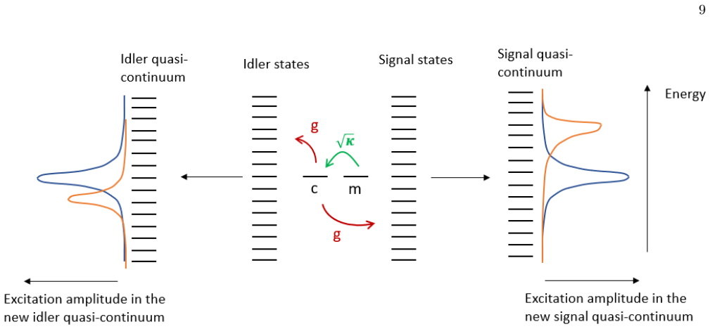
The load-bearing object is the finite covariance matrix $\Theta$ of the bosonic modes—signal, idler, cavity, and material—with the joint spectral amplitude entered as the off-diagonal signal-idler block of the input covariance. Its time evolution is the Sylvester/Lyapunov equation $d\Theta/dt = W\Theta + \Theta W^{\dagger}$, where $W$ is the dynamical matrix from the linearized Heisenberg equations; taking the Laplace transform at $z = 0$ converts the two-time boundary problem into an algebraic one, and the Møller scattering matrix $S = (W^{\dagger} - z)(W - z)^{-1}$ links forward-propagated input modes to backward-propagated output modes. Gaussian preservation is what justifies closing at second moments, so the exponentially large Fock-space simulation is replaced by finite matrix algebra.
What would settle it
Evolve the exact two-photon wavefunction for a single signal-idler pair through the same dynamical matrix W and compare the exact output joint spectral intensity with the prediction of Eq. (30); any discrepancy in the off-diagonal correlation structure would show the Gaussian covariance representation does not carry the single-pair entanglement. A sharper test: prepare two input states with identical joint spectral intensity but different spectral phases—the model's output depends on those phases through F(ωs,ωi) in the initial covariance matrix, so a measurement distinguishing the outputs would settle whether the mapping is physical.
Extended reading notes
Core claim
The central discovery is that a single pair of frequency-entangled photons can be treated as a Gaussian state for the purpose of computing output spectra: the bilinear Hamiltonian makes the evolution Gaussian-preserving, so Wick contractions close the equations of motion at the level of first and second moments. Eq. (30) then expresses the output covariance at t→+∞ directly in terms of the input covariance at t→−∞, the dynamical matrix W, and the scattering matrix S built from forward-propagated input and backward-propagated output modes. Encoding the joint spectral amplitude F(ωs,ωi) in the off-diagonal entries of the input covariance matrix, the model outputs a joint spectral intensity that shifts toward the cavity resonance, narrows like a cavity filter, and develops off-diagonal peaks as the cavity–material coupling grows. These peaks are interpreted as the decay of discrete cavity/material excitations into the signal-idler quasi-continua, producing Lorentzian lineshapes that can become Fano-asymmetric under detuned material coupling. The output entanglement entropy decreases with coupling—faster for a dimer than a monomer—before an upturn at strong coupling signals revived signal-idler correlations.
Load-bearing premise
The whole mapping rests on treating a single photon-pair Fock state as a Gaussian state whose covariance matrix carries the joint spectral amplitude in its off-diagonal entries, even though a single-pair Fock state's true covariance is vacuum-like and does not encode that amplitude.
Editorial extensions
If this is right
- The output joint spectral intensity can be computed from the input joint spectral amplitude by finite matrix algebra, so spectroscopy simulations no longer scale with the exponentially growing Fock space of signal and idler modes.
- Cavity decay leaves a specific fingerprint—off-diagonal peaks in the output JSI—that can be read as a measure of cavity–material coupling strength.
- The output entanglement entropy decreases monotonically with coupling and falls faster for a dimer than a monomer, with a strong-coupling revival; measuring this entropy change gives a direct probe of material correlations.
- Purity and mutual information of the output biphoton state follow from the determinant of the output covariance matrix through the Wigner function, giving closed-form observables beyond the spectrum.
- The framework extends to Tavis-Cummings-type many-body material limits, since any number of material modes keeps the Hamiltonian bilinear and the dynamics Gaussian-preserving.
Reading between the lines
- Because Eq. (30) is an explicit linear map from input covariance to output covariance, it could be inverted against measured output JSIs to reconstruct the phase of the input JSA—an effective phase-retrieval scheme the paper does not pursue.
- The Fano-asymmetry prediction is directly testable by detuning the material mode relative to the cavity; asymmetric off-diagonal peaks would confirm the quasi-continuum decay picture, while their absence would point to a different decoherence mechanism.
- The same Gaussian covariance machinery should apply to multi-photon Gaussian inputs such as two-mode squeezed states, so the Lyapunov map may extend beyond single biphoton pairs to broadband quantum light scattering.
- The paper itself notes the bilinear form excludes pure dephasing, non-Markovian dynamics, and multi-photon interactions; adding pure-dephasing jump operators and checking whether the covariance equations still close would mark the boundary of the Gaussian approximation.
Signed reviews
Editorial analysis
A structured set of objections, weighed in public.
Referee Report
Summary. The manuscript proposes a Lyapunov-based input–output formalism for entangled biphotons interacting with cavity and material modes. It defines a bilinear Hamiltonian, a dynamical matrix W for a mode vector x = (b_s, b_i, a, S), and a covariance matrix Θ = ⟨xx†⟩ − ⟨x⟩⟨x†⟩; by solving Sylvester equations with Møller operators it derives Eq. (30), claimed to map the input covariance at t → −∞ to the output covariance at t → +∞. The framework is then discretized over a signal/idler frequency grid, and the output joint spectral intensity (JSI) is computed for a squeezed Gaussian input and for an experimental SPDC input, showing a resonance-shifted JSI and off-diagonal peaks. The paper also computes output entropy and purity from the covariance matrix.
Significance. The intended goal—a scalable map from input JSA to output JSI that avoids exponentially large Hilbert spaces—is well motivated, and providing public code and a covariance-based target are strengths. If Eq. (30) and the Gaussian covariance representation were valid, the method would offer a useful tool for quantum spectroscopy. However, the central derivation is not sound: the input single-pair Fock state is not correctly represented by Eq. (32), the Laplace-transform step in Eq. (28) is invalid, and Eq. (29) contains a sign error. These are load-bearing issues, so the claimed input-to-output mapping and the resulting figures do not follow from the stated model.
major comments (5)
- [Section II.B, Eqs. (15) and (32)] The matrix in Eq. (32) is not the covariance of the stated input state. For the single-pair Fock state |ψ⟩_in of Eq. (2), the expectation ⟨b_s(ω_s) b_i†(ω_i)⟩ vanishes: annihilating the signal photon leaves a one-idler state, and acting with b_i† creates a two-idler component orthogonal to the original single-idler state; the anomalous moments ⟨b_s b_i⟩ also vanish. Thus the off-diagonal F entries in Eq. (32) do not follow from the definition in Eq. (15), and propagating Eq. (32) does not propagate the biphoton state described by Eq. (2).
- [Section II.B, Eqs. (28)–(29)] The identity ̃x(z) · ̃x(z)† = ̃Θ(z) in Eq. (28) is invalid because the Laplace transform of a product is a convolution, not the product of Laplace transforms. Consequently the covariance transformation ̃Θ_out = −S ̃Θ_in S† does not follow. Moreover, Eq. (27) gives x_out = −S x_in, so the covariance must transform as ̃Θ_out = +S ̃Θ_in S†; the extra minus sign in Eq. (29) is inconsistent with the authors' own mode relation.
- [Section II.B, Eq. (24)] Equation (24) is an identity obtained by combining Eqs. (22) and (23), not a solution: it still contains ̃Θ_out on the right-hand side. Since Eq. (29) is independently invalid, Eq. (30) is left unsupported as the governing equation of the method.
- [Section III.B, Figs. 3–4] The procedure for converting the propagated covariance Θ_out into the plotted JSI is never defined. The text states that the JSI is obtained by tracing out the signal–idler submatrix, but the JSI is |F_out|² and F_out is never related to Θ_out; without this step, the claimed JSA-to-JSI mapping is not a closed calculation.
- [Section III.B] The claimed agreement with the experimental JSI is not a falsifiable test as presented, because the cavity and material frequencies are set to the experimentally observed idler resonance (Fig. 3 caption, Section III.B) and no quantitative comparison, such as a residual, fidelity, or uncertainty estimate, is given; the observed shift is therefore largely a consequence of the chosen resonant filtering.
minor comments (5)
- [Eq. (1)] Equation (1) uses the single symbol b_{s/i}(ω) for both signal and idler modes, which makes the creation/annihilation ordering in Eq. (2) ambiguous; please use distinct labels b_s and b_i throughout.
- [Eq. (14)] Equation (14) introduces −√κ couplings between the cavity and material modes without showing the Heisenberg-equation derivation from the last term of Eq. (1); please spell out the equations of motion.
- [References] The citation to Kinsner [35] for the Lyapunov equation is unconventional; a standard control-theory or quantum-optics reference would be more appropriate.
- [Section III.B] The statement that the result is in close agreement with the experimental study lacks a quantitative comparison metric; please state the measure of agreement.
- [Throughout] There are minor typographical errors, including "occuring" in Section III.B and inconsistent use of "eigenvalues" versus "singular values" after Eq. (33).
Circularity Check
Benchmark prediction is forced by resonance parameters chosen from the target data; core Lyapunov map is otherwise a forward model.
-
fitted input called prediction
[Section III.B (Results, Experimental Initial JSI) and Summary]
"Since the system is set up such that the cavity and material dispersions are nearly in resonance with the idler wavelength (≈ 681nm), these energies are preferentially absorbed by the cavity and material with a higher probability as compared to the signal photons. ... Our simulations predict a shift in the output JSI that is consistent with the experimental observations."
The cavity and material frequencies are chosen to sit on the idler resonance read from the experimental output JSI used for comparison; the predicted shift and the filtering/squeezing of the output JSI are a direct consequence of that choice. The agreement with Ref. [15] is therefore a consistency check of the imposed resonance condition, not an independent prediction generated by the Lyapunov map. The output JSI is the input JSA (placed in the covariance matrix via Eq. (32)) propagated through this chosen filter, so the benchmark does not validate the map against data outside the fitted inputs.
full rationale
The central derivation, Eq. (30), follows algebraically from the Lyapunov/Sylvester equations and the Møller-operator ansatz; it is not circular because the output covariance is a nontrivial function of the dynamical matrix W and the input covariance. The placement of the JSA into the off-diagonal block of Θin (Eq. 32) is an input assumption, and the skeptic's concern that this may not match the covariance of the Fock state in Eq. (15) is a correctness/validity problem rather than a circular reduction. The circularity that is present is confined to the benchmark: the cavity and material frequencies are set to the experimentally observed idler resonance, and the resulting output shift is then reported as a 'prediction' consistent with the same experiment. This makes the validation partially self-fulfilling, though the general Lyapunov map retains independent content. The self-citation [10] used to interpret entanglement entropy is not load-bearing for the map.
Assumptions & free parameters
free parameters (4)
- Cavity frequency omega_c =
1809 meV in Fig. 3
- Material frequency Omega =
1809 meV in Fig. 3
- Cavity-material coupling sqrt(kappa) =
Varied; 488 meV in Fig. 3
- Signal/idler-cavity coupling g =
Not specified
assumptions (5)
- domain assumption The Hamiltonian is bilinear and the evolution preserves Gaussian states (rotating wave and first Markov approximations).
- ad hoc to paper The single-pair biphoton state can be represented by a Gaussian covariance matrix with off-diagonal entries equal to the joint spectral amplitude (Eq. 32).
- ad hoc to paper The Laplace transform of the product of mode vectors equals the product of their Laplace transforms (Eq. 28).
- domain assumption Setting the Laplace variable z = 0 yields time-integrated covariances that satisfy the Lyapunov boundary conditions (Eqs. 22-23).
- domain assumption W_out = W† propagates the moments backward in time (Eq. 26).
Cite this review
Pith. "Pith review of Lyapunov Dynamics in Entangled Biphoton Spectroscopy." pith.science (2026). https://pith.science/paper/DQ2Y32VG
@misc{pith2026250414086,
  author       = {Pith},
  title        = {Pith review of: Lyapunov Dynamics in Entangled Biphoton Spectroscopy},
  year         = {2026},
  howpublished = {\url{https://pith.science/paper/DQ2Y32VG}},
  note         = {Machine review of arXiv:2504.14086}
}
read the original abstract
We develop a Lyapunov-based framework to model the evolution of entangled biphotons interacting with cavity and material modes. Using Gaussian-preserving dynamics and M{\o}ller operators, we map input joint spectral amplitudes to experimentally measurable joint spectral intensities. Our model reproduces key features of observed spectra and reveals off-diagonal correlations arising from cavity decay, providing a scalable and tractable tool for quantum spectroscopic analysis.
Figures


Figures from the paper (3 more)


Reference graph
Works this paper leans on
-
[1]
in terms of ˜Θin(z = 0). For this, we go back to Eq. (13) and take its Laplace transform, z.˜x(z)−xin(t→−∞ ) =Win˜x(z) (25) where Win =W is the dynamical matrix responsible for propagating the vector of moments forward in time from t→−∞ . To connect this to the moments att→ +∞, we defineWout =W† and propagate the moments backward in time using the Laplace...
-
[2]
S. Mukamel, M. Freyberger, W. Schleich, M. Bellini, A. Zavatta, G. Leuchs, C. Silberhorn, R. W. Boyd, L. L. S´ anchez-Soto, A. Stefanov,et al. , Journal of physics B: Atomic, molecular and optical physics 53, 072002 (2020)
work page 2020
- [3]
-
[4]
F. Schlawin and S. Mukamel, The Journal of chemical physics 139 (2013)
work page 2013
-
[5]
K. E. Dorfman, F. Schlawin, and S. Mukamel, Reviews of Modern Physics 88, 045008 (2016)
work page 2016
- [6]
-
[7]
O. Roslyak, C. A. Marx, and S. Mukamel, Physical Re- view A—Atomic, Molecular, and Optical Physics 79, 033832 (2009)
work page 2009
-
[8]
F. Schlawin, K. E. Dorfman, B. P. Fingerhut, and S. Mukamel, Physical Review A—Atomic, Molecular, and Optical Physics 86, 023851 (2012)
work page 2012
Show all 39 references
-
[9]
Schlawin, K
F. Schlawin, K. E. Dorfman, B. P. Fingerhut, and S. Mukamel, Nature communications 4, 1782 (2013)
2013
-
[10]
Upton, M
L. Upton, M. Harpham, O. Suzer, M. Richter, S. Mukamel, and T. Goodson III, The Journal of Physical Chemistry Letters 4, 2046 (2013)
2013
-
[11]
E. R. Bittner, H. Li, A. Piryatinski, A. R. Srimath Kan- dada, and C. Silva, The Journal of Chemical Physics 152 (2020)
2020
-
[12]
H. Li, A. Piryatinski, J. Jerke, A. R. S. Kandada, C. Silva, and E. R. Bittner, Quantum Science and Tech- nology 3, 015003 (2017)
2017
-
[13]
H. Li, A. Piryatinski, A. R. Srimath Kandada, C. Silva, and E. R. Bittner, The Journal of chemical physics 150 (2019)
2019
-
[14]
Debnath and A
A. Debnath and A. Rubio, Frontiers in Physics 10, 879113 (2022)
2022
-
[15]
Cuevas, J
´A. Cuevas, J. C. L´ opez Carre˜ no, B. Silva, M. De Giorgi, D. G. Su´ arez-Forero, C. S´ anchez Mu˜ noz, A. Fieramosca, F. Cardano, L. Marrucci, V. Tasco, et al. , Science Ad- vances 4, eaao6814 (2018)
2018
-
[16]
Malatesta, L
R. Malatesta, L. Uboldi, E. J. Kumar, E. Rojas-Gatjens, L. Moretti, A. Cruz, V. Menon, G. Cerullo, and A. R. S. Kandada, arXiv preprint arXiv:2309.04751 (2023)
2023 arXiv
-
[17]
Moretti, E
L. Moretti, E. Rojas-Gatjens, L. Uboldi, D. O. Tiede, E. J. Kumar, C. Trovatello, F. Preda, A. Perri, C. Man- zoni, G. Cerullo, et al., The Journal of Chemical Physics 159 (2023)
2023
-
[18]
H. Deng, H. Haug, and Y. Yamamoto, Reviews of modern physics 82, 1489 (2010)
2010
-
[19]
Kasprzak, M
J. Kasprzak, M. Richard, S. Kundermann, A. Baas, P. Jeambrun, J. M. J. Keeling, F. Marchetti, M. Szyma´ nska, R. Andr´ e, J. Staehli,et al. , Nature 443, 409 (2006)
2006
-
[20]
Keeling and S
J. Keeling and S. K´ ena-Cohen, Annual Review of Physi- cal Chemistry 71, 435 (2020)
2020
-
[21]
A. Amo, J. Lefr` ere, S. Pigeon, C. Adrados, C. Ciuti, I. Carusotto, R. Houdr´ e, E. Giacobino, and A. Bramati, Nature Physics 5, 805 (2009)
2009
-
[22]
Lerario, A
G. Lerario, A. Fieramosca, F. Barachati, D. Ballarini, K. S. Daskalakis, L. Dominici, M. De Giorgi, S. A. Maier, G. Gigli, S. K´ ena-Cohen,et al. , Nature Physics 13, 837 (2017)
2017
-
[23]
Amthor, T
M. Amthor, T. C. Liew, C. Metzger, S. Brodbeck, L. Worschech, M. Kamp, I. A. Shelykh, A. V. Kavokin, C. Schneider, and S. H¨ ofling, Physical Review B 91, 081404 (2015)
2015
-
[24]
Pickup, K
L. Pickup, K. Kalinin, A. Askitopoulos, Z. Hatzopoulos, P. Savvidis, N. G. Berloff, and P. Lagoudakis, Physical review letters 120, 225301 (2018)
2018
-
[25]
Dorfman, S
K. Dorfman, S. Liu, Y. Lou, T. Wei, J. Jing, F. Schlawin, and S. Mukamel, Proceedings of the National Academy of Sciences 118, e2105601118 (2021)
2021
-
[26]
M. Sich, D. V. Skryabin, and D. N. Krizhanovskii, Comptes Rendus. Physique 17, 908 (2016)
2016
-
[27]
Grosso, G
G. Grosso, G. Nardin, F. Morier-Genoud, Y. L´ eger, and B. Deveaud-Pl´ edran, Physical review letters107, 245301 (2011)
2011
-
[28]
Klembt, T
S. Klembt, T. Harder, O. Egorov, K. Winkler, R. Ge, M. Bandres, M. Emmerling, L. Worschech, T. Liew, M. Segev, et al. , Nature 562, 552 (2018)
2018
-
[29]
Karzig, C.-E
T. Karzig, C.-E. Bardyn, N. H. Lindner, and G. Refael, Physical Review X 5, 031001 (2015)
2015
-
[30]
H. Wang, A. Kumar, S. Dai, X. Lin, Z. Jacob, S.-H. Oh, V. Menon, E. Narimanov, Y. D. Kim, J.-P. Wang, et al. , Nature communications 15, 69 (2024)
2024
-
[31]
Fang and Y
W. Fang and Y. Yang, Optics Express 28, 32955 (2020)
2020
-
[32]
Nemilentsau, T
A. Nemilentsau, T. Low, and G. Hanson, Physical review letters 116, 066804 (2016). 11
2016
-
[33]
C. W. Gardiner and M. J. Collett, Physical Review A 31, 3761 (1985)
1985
-
[34]
Gardiner and P
C. Gardiner and P. Zoller, Quantum Noise, Springer- Verlag, Berlin (2004)
2004
-
[35]
Bouchard, A
F. Bouchard, A. Sit, Y. Zhang, R. Fickler, F. M. Miatto, Y. Yao, F. Sciarrino, and E. Karimi, Reports on Progress in Physics 84, 012402 (2020)
2020
-
[36]
Kinsner, IEEE Transactions on Systems, Man, and Cybernetics, Part C (Applications and Reviews) 36, 141 (2006)
W. Kinsner, IEEE Transactions on Systems, Man, and Cybernetics, Part C (Applications and Reviews) 36, 141 (2006)
2006
-
[37]
Møller, Nature 158, 403 (1946)
C. Møller, Nature 158, 403 (1946)
1946
-
[38]
Ferraro, S
A. Ferraro, S. Olivares, and M. G. Paris, arXiv preprint quant-ph/0503237 (2005)
2005 arXiv
-
[39]
Cohen-Tannoudji, J
C. Cohen-Tannoudji, J. Dupont-Roc, and G. Grynberg, Atom-photon interactions: basic processes and applica- tions (John Wiley & Sons, 1998)
1998
Reviewed August 16, 2026 · model on record in the stance chip above.
Discussion (0). Continue with ORCID to comment.