REVIEW 2 major objections 5 minor 25 references
Least-Squares-Embedded Optimization for Accelerated Convergence of PINNs in Acoustic Wavefield Simulations
T0 review · 2 major / 5 minor · reviewed 2026-08-16 · deepseek-v4-flash
Pith's one-line read A least-squares solve for the output layer, embedded into the PINN loss, makes scattered-wavefield Helmholtz training converge fast and stably where plain gradient descent stalls.
desk verdict Non-PML LS-embedding for PINN Helmholtz is a clean incremental contribution; the PML half has a load-bearing matrix bug and the Marmousi results need re-running before they can be trusted. read the letter →
The pith
A machine-rendered reading of the paper's core claim, the machinery that carries it, and where it could break.
The reading
What carries the argument
The load-bearing object is the least-squares-embedded loss $L = \sum_j |DW^* - R|^2$ of Eq. 22. Here $D$ is a matrix assembled from the PDE residual operator acting on the penultimate-layer outputs $H$ and from the source soft-constraint term; $R$ contains the background-wavefield forcing; and $W^*$ is the damped least-squares output weight from Eq. 21. The mechanism is that each training step solves the small $P \times P$ normal system $(D^T D + \epsilon I)W^* = D^T R$ by Cholesky decomposition, then propagates gradients of this loss through $W^*$ back to the hidden layers using automatic differentiation, with forward-mode differentiation providing the derivatives of $H$ efficiently. This turns the linear output layer into an exactly solved subproblem and leaves gradient descent with only the nonlinear hidden features to learn.
What would settle it
Compute, at a fixed epoch of the published code, the Eq. 22 loss using the Eq. 25 matrix and compare it with the sum of the PML PDE residual (Eq. 12) and $\beta$ times the soft constraint (Eq. 13) on the same wavefield; if the soft-constraint contribution equals $\|D_C(W_r+W_i)\|^2$ rather than $\|D_C W_r\|^2+\|D_C W_i\|^2$, the PML experiments minimize a different objective and the paper's PML claim is not established.
Extended reading notes
Core claim
The central discovery is that the loss function for PINN training can be redefined as $L = \sum_j |DW^* - R|^2$, where $W^* = (D^T D + \epsilon I)^{-1} D^T R$ is the damped least-squares solution for the output weights given the current penultimate-layer features $H$. Because $W^*$ is the exact minimizer of the quadratic PDE-plus-constraint loss for the output layer, every gradient-descent step optimizes the hidden layers against the best possible linear readout rather than a readout partway through a gradient trajectory. The paper derives $D$ and $R$ for the scattered Helmholtz equation in two settings: with real and imaginary parts decoupled when no perfectly matched layer is used, and with a block matrix that couples them when PML coordinate stretching is included. The numerical claim is that this change alone, with no architectural modification, makes 10 Hz and 30 Hz scattered wavefield PINNs converge rapidly and stably, even with 500 collocation points or only 8 penultimate neurons, where standard GD training stalls.
Load-bearing premise
The method assumes the PML soft-constraint term can be written as one shared block applied to the sum of the real and imaginary wavefield parts, but the written penalty requires separate blocks on each part; if the implementation follows the matrix in Eq. 25, the Marmousi training optimizes a different objective than the paper states, and the reported PML convergence would not demonstrate the claimed loss.
Editorial extensions
If this is right
- With the LS-embedded loss, the PINN converges from the first epochs even with very few collocation points, so the number of collocation points required per epoch can be drastically reduced compared to plain GD training.
- The method consistently achieves lower validation error than standard GD on the simple velocity model across different collocation counts and different penultimate layer widths, including widths as small as 8 neurons.
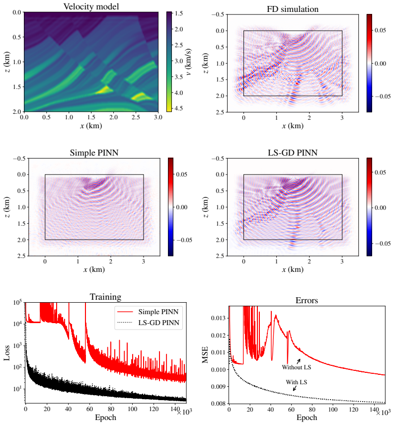
- In the Marmousi 30 Hz test with PML, the LS-GD method reaches in about 15,000 epochs an accuracy that plain GD does not reach after 150,000 epochs, and it does so with markedly smaller loss fluctuations.
- The added computational cost of the LS step is modest, scaling as $O((N+N_C)P^2)$ to assemble the normal matrix and $O(P^3)$ for the Cholesky solve, where $P$ is the penultimate layer width.
- The same loss reformulation applies both with and without perfectly matched layers, so the training upgrade can be used in realistic absorbing-boundary seismic simulations.
Reading between the lines
- Editorial inference: The same loss reformulation should transfer to any PDE residual that is linear in a final linear network layer, such as time-harmonic elasticity, diffusion, or Maxwell-type equations, where the LS step would be a drop-in change to the training loop.
- Editorial inference: Because the LS solve removes the output-layer coordinates from the GD landscape, the hidden layers become the sole nonlinear feature learners; one testable expectation is that architecture choices such as depth, width, and activation will matter more under LS-GD than under plain GD.
- Editorial inference: The method's per-batch exact solves also suggest a natural combination with adaptive sampling: if collocation batches are chosen to emphasize high-residual regions, the LS output layer will reflect that emphasis immediately, potentially making the method more responsive than GD to adaptive collocation strategies.
Signed reviews
Editorial analysis
A structured set of objections, weighed in public.
Referee Report
Summary. The paper proposes a hybrid least-squares/gradient-descent (LS-GD) training scheme for physics-informed neural networks (PINNs) solving the frequency-domain scattered Helmholtz equation. The key idea is to replace the standard gradient-descent update of the linear output layer with an analytic damped least-squares solve, and to define the GD loss as the residual of that solve (Eq. 22), so that the hidden layers are trained against the optimal output layer at each iteration. Derivations are given for the case without PML (Eqs. 17-20) and with PML (Eqs. 23-25), together with implementation details and complexity estimates. Numerical experiments on a 10 Hz simple model and a 30 Hz Marmousi model compare the proposed LS-GD training with standard GD training of the same network architecture.
Significance. The non-PML least-squares derivation is mathematically sound, and the single-loss embedding is a clean variant of the alternating LS/GD schemes of Cyr et al. and Uriarte et al.; if the PML formulation is corrected, the paper would provide a practically useful and low-overhead acceleration for PINN-based Helmholtz solvers. The reported experiments show large qualitative improvements in convergence on benchmark models, and the promise of released code is a strength. However, the PML block in Eq. 25 does not implement the stated soft constraint, and because the Marmousi experiment uses Eq. 25, the current evidence for the PML half of the central claim is compromised. The contribution is incremental rather than a new optimization paradigm, but it is a meaningful one for wavefield simulation applications.
major comments (2)
- [Section 2.4.2, Eq. (25)] The third block row [D_C, D_C] of the PML least-squares matrix does not implement the soft constraint in Eq. 13. With the output weights stacked as W = [W_r; W_i], this block contributes ||D_C(W_r + W_i)||^2 = (β/N_C) Σ_j γ_j^2 (u_{r,j} + u_{i,j})^2 to the LS objective, whereas Eq. 13 requires (β/N_C) Σ_j γ_j^2 (u_{r,j}^2 + u_{i,j}^2). The correct representation is block-diagonal [D_C, 0; 0, D_C]. As printed, the LS problem minimizes a different objective that includes a spurious cross-term 2(β/N_C)Σ_j γ_j^2 u_{r,j} u_{i,j}. Since the Marmousi experiment (Section 4.2) uses Eqs. 22 and 25, its reported loss and MSE curves are evidence for the stated loss only if the released code actually uses the corrected block and the text is merely misprinted. Please fix the matrix, rerun the PML experiments, and state explicitly which form the code implements.
- [Section 4, Figs. 3-5] The abstract and conclusion claim that the LS solver adds minimal computational overhead and that the method converges where standard GD fails, but no wall-clock times, per-epoch costs, or multiple-seed statistics are reported. The complexity analysis in Section 5 counts only the normal-matrix construction and Cholesky solve; it does not account for the cost of building D by forward-mode differentiation at every epoch or for backpropagating through the LS solve when training the hidden layers. Please report runtimes or measured per-epoch costs for the reported experiments and, for the claim that standard GD 'fails' on Marmousi, repeat the comparison with at least a few random seeds so the reader can assess robustness.
minor comments (5)
- [Eq. (16) and Eq. (21)] Equation 16 introduces W without specifying its dimensions or relation to the later W*; please clarify that W here denotes the output-layer weight matrix, while W* in Eq. 21 is the damped least-squares solution used in the loss of Eq. 22.
- [Section 2.3, Eq. (14)] The wavelength λ is not defined in the text; if it denotes the acoustic wavelength, please state the corresponding frequency and reference velocity used to evaluate it.
- [Section 3] Please state explicitly whether the gradient of the loss in Eq. 22 flows through the damped LS solve W* = (D^T D + εI)^{-1} D^T R or whether W* is treated as a detached constant; this is important for reproducing the reported training dynamics.
- [Figure 5(f) and Section 4.2] The validation MSE is reported excluding the PML region; this exclusion is mentioned only in the figure caption and should be stated in the main text, together with a justification for omitting the PML zone from the reported error.
- [Throughout] Please correct the typos: 'itterative' (Section 2.4.1), 'trianing' and 'gradualy' (Section 3), 'expriments' (Section 5), and 'oberved' (Section 4.1).
Circularity Check
No circularity found: the LS output-layer solve is derived from current network features, and same-author citations supply only problem inputs.
full rationale
The derivation chain for the central claim is self-contained. The least-squares step computes W* = (D^T D + epsilon I)^-1 D^T R from the current penultimate-layer features H, and the GD loss L = sum |D W* - R|^2 is then minimized over the hidden-layer parameters. This is exactly the proposed hybrid algorithm, and the 'optimal update' for the linear output layer is a direct algebraic consequence of solving the normal equations, not an imported conclusion. The same-author citations (Abedi et al. 2025; Alkhalifah et al. 2021; Huang and Alkhalifah 2023) supply the PML Helmholtz form, the analytic background wavefield, and the soft-constraint idea; these are problem inputs applied symmetrically to both the simple PINN and the LS-GD PINN, and none of them asserts the convergence or accuracy results. The numerical evidence is checked against finite-difference reference solutions, which are external benchmarks. A possible algebraic mismatch in the PML block row of Eq. (25) (printed [DC, DC] versus block-diagonal [DC, 0; 0, DC] for the constraint term) is a correctness concern about which objective is actually minimized, not a circularity: even if the printed matrix is wrong, the derivation does not assume its own conclusion. No prediction reduces to a fitted parameter, to a self-citation chain, or to a definition of the target quantity.
Assumptions & free parameters
free parameters (4)
- Tikhonov regularization ε =
0.1 initially, reduced toward 1e-4
- Constraint weight β =
Not specified numerically
- Learning rate schedule =
0.002 decaying to ~0.0007
- PML damping scale a0 =
0.8 (Marmousi)
assumptions (5)
- domain assumption The scattered Helmholtz equation (Eq 1) governs the scattered acoustic wavefield.
- domain assumption The PML-stretched equation (Eq 2) with stretching factors (Eq 3) correctly absorbs outgoing waves.
- domain assumption The analytical background wavefield u0 (Eq 6) is exact inside the domain and a sufficiently accurate approximation in the PML region.
- standard math Setting the output-layer weights to the damped least-squares solution W* and descending ||DW* - R||² provides valid, unbiased gradient directions for the hidden layers.
- ad hoc to paper The soft constraint (Eq 13) can be embedded as a linear least-squares block in D.
Cite this review
Pith. "Pith review of Least-Squares-Embedded Optimization for Accelerated Convergence of PINNs in Acoustic Wavefield Simulations." pith.science (2026). https://pith.science/paper/PIUA45WT
@misc{pith2026250416553,
  author       = {Pith},
  title        = {Pith review of: Least-Squares-Embedded Optimization for Accelerated Convergence of PINNs in Acoustic Wavefield Simulations},
  year         = {2026},
  howpublished = {\url{https://pith.science/paper/PIUA45WT}},
  note         = {Machine review of arXiv:2504.16553}
}
read the original abstract
Physics-Informed Neural Networks (PINNs) have shown promise in solving partial differential equations (PDEs), including the frequency-domain Helmholtz equation. However, standard training of PINNs using gradient descent (GD) suffers from slow convergence and instability, particularly for high-frequency wavefields. For scattered acoustic wavefield simulation based on Helmholtz equation, we derive a hybrid optimization framework that accelerates training convergence by embedding a least-squares (LS) solver directly into the GD loss function. This formulation enables optimal updates for the linear output layer. Our method is applicable with or without perfectly matched layers (PML), and we provide practical tensor-based implementations for both scenarios. Numerical experiments on benchmark velocity models demonstrate that our approach achieves faster convergence, higher accuracy, and improved stability compared to conventional PINN training. In particular, our results show that the LS-enhanced method converges rapidly even in cases where standard GD-based training fails. The LS solver operates on a small normal matrix, ensuring minimal computational overhead and making the method scalable for large-scale wavefield simulations.
Figures


Figures from the paper (2 more)

Reference graph
Works this paper leans on
-
[1]
Gabor-Enhanced Physics-Informed Neural Networks for Fast Simulations of Acoustic Wavefields
Abedi, M. M., Pardo, D., and Alkhalifah, T. (2025). Gabor-enhanced physics-informed neural networks for fast simulations of acoustic wavefields. arXiv preprint arXiv:2502.17134
work page Pith review arXiv 2025
-
[2]
Alkhalifah, T., Song, C., bin Waheed, U., and Hao, Q. (2021). Wavefield solutions from machine learned functions constrained by the Helmholtz equation. Artificial Intelligence in Geosciences , 2:11–19
work page 2021
-
[3]
Baharlouei, S., Taylor, J. M., Uriarte, C., and Pardo, D. (2025). A least-squares-based neural network (LS-Net) for solving linear parametric PDEs. Computer Methods in Applied Mechanics and Engineering , 437:117757
work page 2025
-
[4]
Berenger, J.-P. (1994). A perfectly matched layer for the absorption of electromagnetic waves. Journal of computational physics, 114(2):185–200
work page 1994
-
[5]
Bihlo, A. (2024). Improving physics-informed neural networks with meta-learned optimization. Journal of Machine Learning Research, 25(14):1–26
work page 2024
-
[6]
S., Giampaolo, F., Rozza, G., Raissi, M., and Piccialli, F
Cuomo, S., Di Cola, V. S., Giampaolo, F., Rozza, G., Raissi, M., and Piccialli, F. (2022). Scientific machine learning through physics–informed neural networks: Where we are and what’s next. Journal of Scientific Computing, 92(3):88
work page 2022
-
[7]
Cyr, E. C., Lan, Y., and Xu, J. (2020). Physics-informed neural networks using a hybrid least-squares and gradient descent optimization approach. SIAM Journal on Scientific Computing , 42(4):A2504–A2531
work page 2020
-
[8]
El-Sayed, S. M. and Kaya, D. (2004). Comparing numerical methods for Helmholtz equation model problem. Applied Mathematics and Computation , 150(3):763–773
work page 2004
Show all 25 references
-
[9]
and Alkhalifah, T
Huang, X. and Alkhalifah, T. (2023). GaborPINN: Efficient physics informed neural networks using multi- plicative filtered networks. IEEE Geoscience and Remote Sensing Letters
2023
-
[10]
Huang, X., Alkhalifah, T., and Song, C. (2021). A modified physics-informed neural network with positional encoding. In SEG International Exposition and Annual Meeting , page D011S106R002. SEG
2021
-
[11]
Neal, B., Mittal, S., Baratin, A., Tantia, V., Scicluna, M., Lacoste-Julien, S., and Mitliagkas, I. (2018). A modern take on the bias-variance tradeoff in neural networks. arXiv preprint arXiv:1810.08591
2018 arXiv
-
[12]
Pratt, R. G. (1999). Seismic waveform inversion in the frequency domain, part 1: Theory and verification in a physical scale model. Geophysics, 64(3):888–901
1999
-
[13]
Raissi, M., Perdikaris, P., and Karniadakis, G. E. (2019). Physics-informed neural networks: A deep learning framework for solving forward and inverse problems involving nonlinear partial differential equations. Journal of Computational Physics , 378:686–707. 12
2019
-
[14]
Sirgue, L., Etgen, J., and Albertin, U. (2008). 3D frequency domain waveform inversion using time domain finite difference methods. In 70th EAGE Conference and Exhibition incorporating SPE EUROPEC 2008 , pages cp–40. European Association of Geoscientists & Engineers
2008
-
[15]
Song, C., Alkhalifah, T., and Waheed, U. B. (2021). Solving the frequency-domain acoustic VTI wave equation using physics-informed neural networks. Geophysical Journal International, 225(2):846–859
2021
-
[16]
and Wang, Y
Song, C. and Wang, Y. (2023). Simulating seismic multifrequency wavefields with the fourier feature physics- informed neural network. Geophysical Journal International, 232(3):1503–1514
2023
-
[17]
M., and Rojas, S
Uriarte, C., Bastidas, M., Pardo, D., Taylor, J. M., and Rojas, S. (2025). Optimizing variational physics- informed neural networks using least squares. Computers & Mathematics with Applications , 185:76–93
2025
-
[18]
N., Kaiser, L., and Polosukhin, I
Vaswani, A., Shazeer, N., Parmar, N., Uszkoreit, J., Jones, L., Gomez, A. N., Kaiser, L., and Polosukhin, I. (2017). Attention is all you need. In Proceedings of the 31st International Conference on Neural Information Processing Systems, NIPS’17, page 6000–6010, Red Hook, NY, ...
2017
-
[19]
Versteeg, R. (1994). The Marmousi experience: Velocity model determination on a synthetic complex data set. The Leading Edge, 13(9):927–936
1994
-
[20]
Waheed, U. B. (2022). Kronecker neural networks overcome spectral bias for PINN-based wavefield compu- tation. IEEE Geoscience and Remote Sensing Letters , 19:1–5
2022
-
[21]
S., Operto, S., and Ma, J
Wu, Y., Aghamiry, H. S., Operto, S., and Ma, J. (2023). Helmholtz-equation solution in nonsmooth media by a physics-informed neural network incorporating quadratic terms and a perfectly matching layer condition. Geophysics, 88(4):T185–T202
2023
-
[22]
and Alkhalifah, T
Wu, Z. and Alkhalifah, T. (2018). An efficient Helmholtz solver for acoustic transversely isotropic media. Geophysics, 83(2):C75–C83
2018
-
[23]
Xu, S., Yan, C., Sun, Z., Huang, R., Guo, D., and Yang, G. (2024). On the preprocessing of physics-informed neural networks: How to better utilize data in fluid mechanics. arXiv preprint arXiv:2403.19923
2024 arXiv
-
[24]
and Ma, J
Yang, F. and Ma, J. (2023). Fwigan: Full-waveform inversion via a physics-informed generative adversarial network. Journal of Geophysical Research: Solid Earth , 128(4):e2022JB025493
2023
-
[25]
and Ma, J
Yang, F. and Ma, J. (2025). Gabor-wavelet-activation implicit neural learning for full waveform inversion. Geophysics, 90(3):1–78. 13
2025
Reviewed August 16, 2026 · model on record in the stance chip above.
Discussion (0). Continue with ORCID to comment.