REVIEW 4 major objections 6 minor 1 cited by
Goal-Oriented Time-Series Forecasting: Foundation Framework Design
T0 review · 4 major / 6 minor · reviewed 2026-08-16 · deepseek-v4-flash
Pith's one-line read A forecasting model trained on a grid of value intervals can be redirected to any new interval at inference time without retraining.
desk verdict Solid interval-conditioned forecasting scheme with a useful new dataset, but the 'arbitrary interval' claim needs off-grid experiments and more statistical rigor before it can be accepted at face value. read the letter →
The pith
A machine-rendered reading of the paper's core claim, the machinery that carries it, and where it could break.
The reading
What carries the argument
The load-bearing mechanism is a discretized interval-conditioned training objective over a partition $\mathcal{C}_L$ of the prediction space, combined with two inference-time patching equations. Each training cell carries a soft decay weight $d_\nu(y,I)=\exp(-\nu\max(0,|y-\Delta_{\mathrm{avg}}|-\Delta_{\mathrm{diff}}))$, where $\Delta_{\mathrm{avg}}$ and $\Delta_{\mathrm{diff}}$ are the cell midpoint and half-width; as $\nu\to\infty$ this weight becomes the indicator that $y$ lies in $I$, and for finite $\nu$ it creates soft overlap between neighboring cells. A shared classification head predicts membership of the true value in each cell, and the loss combines regression with the classification term weighted by $\phi$. At inference, the patching map $\Xi_L(I)$ collects the cells intersecting the requested interval, and the final forecast is either the classifier-probability-weighted average of those cells' regression outputs or the output of the single most confident cell. The mechanism matters because each fine cell learns a local conditional expectation rather than the global average, so the model can represent hypotheses that differ sharply across regions of the output space.
What would settle it
Hold out a target interval much narrower than the finest training cell (for instance, the lowest decile of a cell) on a dataset whose conditional distribution inside that cell is strongly non-uniform, train an end-to-end (E2E) model on that narrow interval, and compare its MAE with the patched forecast from $D^\star_L$. If the patched MAE is not close to the E2E MAE, or if the classifier's probability estimates for the intersecting cells deviate systematically from empirical frequencies on a held-out set, then the claim that arbitrary intervals are served without retraining is falsified.
Extended reading notes
Core claim
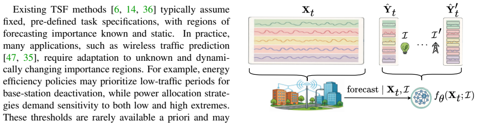
The central discovery is that interval-conditioned forecasting can be split into a discrete training phase and an inference-time patching phase without losing the accuracy of a model trained end-to-end on the target interval itself. During training, the prediction range $\mathcal{X}$ is divided into $L$ disjoint cells, and the model learns, for each cell, a regression forecast $f_\theta(X,I')$ and a classifier $f^c_\theta(X,I')$ estimating the probability that the true future values lie inside that cell. At inference, an arbitrary interval $I$ is served by taking only the cells that intersect it, $\Xi_L(I)=\{I'\in\operatorname{supp}(\mathcal{C}_L): I'\cap I\neq\emptyset\}$, and combining their forecasts either by classifier-weighted averaging or by selecting the most confident cell. The paper reports that this scheme reduces mean absolute error within each region of interest compared with the baseline policy on the synthetic and real-world traces considered, and that it improves decision quality in the downstream energy-saving application by matching the perfect-foresight policy more closely.
Load-bearing premise
The central assumption is that for a newly requested interval, stitching together the pre-trained grid cells that intersect it reproduces what a model trained directly on that interval would predict, which requires the grid to be fine enough relative to the requested interval and the classifier's confidence weights to be well calibrated; the paper itself notes the granularity trade-off in its hyperparameter study but gives no bound on the patching error.
Editorial extensions
If this is right
- A single checkpoint can serve an open-ended family of downstream tasks: any interval requested at inference is answered by patching pre-trained cells, so adapting to a new objective costs no additional training.
- Forecast error inside the application's region of interest drops relative to standard training: the paper reports MAE reductions across DLinear, TimeMixer, PatchTST, and iTransformer on traffic, weather, electricity, and wireless beam-level traces.
- Downstream decisions improve: in the two-tier cell energy-saving experiment, patched forecasts reduce sleep-duration error by about a factor of three, roughly one hour per day, and lower the per-day energy-saving mismatch from 0.950 kW to 337 W.
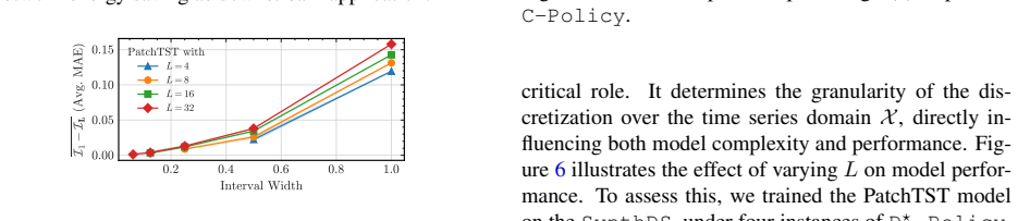
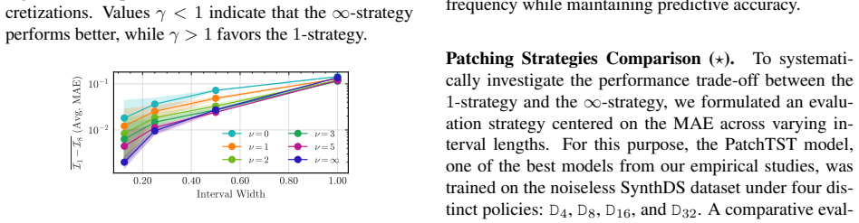
- The number of grid cells $L$ is the key tuning knob: finer grids represent narrower intervals but require more patching, and the paper's sensitivity study shows a granularity-versus-robustness trade-off rather than a monotonic win.
Reading between the lines
- A natural extension is to apply the same cell-and-patch training to existing large time-series foundation models by fine-tuning them on a discretized output grid; the paper names this direction in its conclusion, and success would make interval-adaptive focus a property of foundation models rather than a separate training scheme.
- Because the machinery only needs a partition of the output space and a gate that selects relevant cells, it should generalize to non-interval regions such as quantile bands, regime conditions, or anomaly zones; testing on irregular or overlapping regions would show whether cell patching is the essential ingredient.
- The classifier probabilities play a role like a gating mixture, so a promising check is to measure their calibration on intervals outside the training support; well-calibrated gates would turn the weighted average into something closer to a Bayesian mixture that also reports uncertainty bounds for the patched forecast.
- The reported threefold reduction in sleep-duration error suggests a broader principle: when the downstream loss is asymmetric, a model trained to be locally correct in a movable region can beat a globally optimal forecaster on the decision objective that ultimately matters, going beyond predict-then-optimize by making the region a query rather than a fixed input.
Signed reviews
Editorial analysis
A structured set of objections, weighed in public.
Referee Report
Summary. The manuscript proposes a training methodology for time-series forecasting that aims to make a single model adaptive, at inference time, to application-specified intervals of interest, without retraining. The authors formalize five policies: a baseline (B-Policy), an end-to-end interval-specific policy (E2E-Policy), a continuous-interval sampling policy (C-Policy), a discrete-interval policy (DL-Policy), and a discretized policy with patching (D*_L-Policy) that combines or selects interval-specific predictions via averaging or maximum-confidence selection. The D*_L method uses a soft decay function and an auxiliary classifier to weight interval-specific forecasts. Experiments are conducted on a synthetic trace, a newly released beam-level wireless traffic dataset, and standard benchmarks (Traffic, Electricity, Weather), using iTransformer, DLinear, PatchTST, and TimeMixer. The main metric is MAE within intervals of interest. A downstream energy-saving application for a two-tier wireless network is also presented, and the authors report a threefold reduction in sleep-duration error relative to the baseline. The paper also releases the BLW-TrafficDS dataset and code.
Significance. If the central claims were fully established, the framework would offer a practical path to reconfiguring forecasting models toward different downstream objectives at inference time, a capability relevant to wireless network management, energy optimization, and other decision-focused applications. The paper has clear strengths: a well-defined problem formulation, explicit training objectives for each policy, a newly released dataset, reproducible code, and a sensitivity analysis of the newly introduced hyperparameters (L, nu, delta, patching strategy). The main quantitative claim, however, is currently supported only for target intervals aligned with the training discretization, and the statistical evidence is incomplete. The 'arbitrary interval' and downstream-benefit claims require additional experimental and analytical support before the results can be considered conclusive.
major comments (4)
- [§5, Table 1] Table 1 reports MAE values and improvement percentages without standard deviations or statistical significance tests. Several entries show zero improvement or very small gains (e.g., DLinear I1 on BLW-TrafficDS shows 0.0% improvement, and the overall Electricity improvement for DLinear is 0.7%), so it is not possible to determine whether the reported advantages of D*_L over the baseline are within run-to-run noise. Without variance estimates or paired tests, the central quantitative claim that the proposed policies consistently improve interval-specific accuracy is not established.
- [§4, Eqs. (13)-(15); §5.3.2] The patching mechanism is defined only over the training intervals that intersect the target interval I. If I is strictly contained in a single training interval J, then Ξ_L(I) contains J, and the produced forecast is effectively trained on the loss restricted to all of J, not to the finer target I; the method therefore cannot recover conditional forecasts at a granularity finer than the training grid. The authors acknowledge this trade-off in Section 5.3.2 but do not provide any bound on the approximation error or a calibration analysis for the classifier probabilities fc_θ used as weights in Eq. (14). Moreover, all experiments in Table 1 and Figures 6-7 evaluate intervals aligned with the training discretization (power-of-two partitions), so the abstract's claim of support for 'arbitrary' or 'on-demand' intervals is not tested for off-grid or narrower target intervals.
- [§5.3.1, Figure 5] The downstream energy-saving experiment reports that the task-specific policy reduces sleep-duration error by a factor of three relative to the baseline, but this conclusion is based on a single configuration with no error bars, sensitivity analysis, or statistical comparison. In addition, the forecasting target interval is chosen as [0, 0.5], while the decision thresholds are restricted to U_th in [0, 0.025]; the connection between this broad interval and the threshold distribution is not explained, making it unclear whether the improvement is due to interval-specific training or simply to better overall forecast quality. The authors should provide repeated runs, confidence intervals, and a clearer mapping between the specified interval and the decision thresholds used in the optimization.
- [§5.2, Figure 4] The E2E policy is described as the optimal benchmark that illustrates best-case performance, but it is only shown qualitatively on SynthDS and is not included in Table 1. Because E2E represents the upper bound for inference-time adaptation, its absence from the quantitative comparisons makes it difficult to judge how close D*_L comes to this bound on real-world datasets. Adding E2E results (where feasible) or a clear explanation of why it is excluded would strengthen the evaluation.
minor comments (6)
- [§4, Eq. (10)] The classification loss l'_ν is referred to as 'a classification loss like cross entropy' but is never formally defined; please state the exact form used in the experiments.
- [Table 1] The header row of Table 1 is typeset in a way that interleaves policy names and improvement columns, making it difficult to read; the formatting should be restructured for clarity.
- [Figure 2] The caption refers to 'four intervals' while only I1 and I3 appear in the figure; either display all intervals or adjust the caption to describe what is shown.
- [§4, Eq. (13)] The notation ˙S for the union of disjoint sets is nonstandard; consider using ⊔ or an explicit description to avoid confusion.
- [§5.1, SynthDS description] The text says 'the same randomly selected signal is concatenated multiple times' to generate the trace, but Figure 3a shows four distinct hypotheses; please reconcile the description with the figure.
- [§5.3.1, Eq. (23)] The downstream optimization is over the threshold u_th, but the forecasting model is evaluated with a fixed interval [0, 0.5]; please clarify how the interval specification relates to the threshold distribution used in the decision process.
Circularity Check
No significant circularity: the derivation is self-contained and no fitted quantity is relabeled as a prediction.
full rationale
The paper's proposed D*_L policy trains a forecasting model with an interval-conditioned loss (including a decay-weighted regression term and a classification term) and then combines predictions from training intervals at inference via Eqs. (13)-(15). The final forecast for a target interval I is a function of the trained model outputs, not of the evaluation data or of the target interval's true values; no fitted parameter is renamed as a prediction, and no definitional equivalence forces the result. The patching approximation is an architectural choice with an acknowledged granularity trade-off (Section 5.3.2), meaning some arbitrary intervals may be poorly approximated, but this is a limitation in scope of the evidence, not a circularity. The comparisons against the B-Policy are expected to favor the interval-conditioned models, but that is the intended design rather than a reduction of the claimed result to its inputs. There is no load-bearing self-citation, no uniqueness theorem imported from the authors, and no ansatz smuggled in via citation. The paper is self-contained in the sense required by the circularity analysis: the reported quantities come from trained models and simulations, and the central derivation chain does not reduce to its own assumptions by construction.
Assumptions & free parameters
free parameters (4)
- L (number of discretization intervals) =
8 for BLW-TrafficDS, 4 for other datasets; sensitivity sweeps up to 32
- nu (decay rate) =
varied in {0, 1, 2, 5, ∞} in experiments
- phi (classification loss weight) =
not reported in the text
- delta (interval separation for C-Policy) =
optimal around 5% of the domain
assumptions (3)
- domain assumption The time series values lie in a bounded set X with |X| < ∞
- domain assumption The target interval I is a contiguous value range, and the model can be trained to predict the conditional expectation of Y given X and Y in I
- domain assumption Classifier probabilities fc_theta are usable as weights in the patching combination
Cite this review
Pith. "Pith review of Goal-Oriented Time-Series Forecasting: Foundation Framework Design." pith.science (2026). https://pith.science/paper/E752W6VD
@misc{pith2026250417493,
  author       = {Pith},
  title        = {Pith review of: Goal-Oriented Time-Series Forecasting: Foundation Framework Design},
  year         = {2026},
  howpublished = {\url{https://pith.science/paper/E752W6VD}},
  note         = {Machine review of arXiv:2504.17493}
}
read the original abstract
Conventional time-series forecasting methods typically aim to minimize overall prediction error, without accounting for the varying importance of different forecast ranges in downstream applications. We propose a training methodology that enables forecasting models to adapt their focus to application-specific regions of interest at inference time, without retraining. The approach partitions the prediction space into fine-grained segments during training, which are dynamically reweighted and aggregated to emphasize the target range specified by the application. Unlike prior methods that predefine these ranges, our framework supports flexible, on-demand adjustments. Experiments on standard benchmarks and a newly collected wireless communication dataset demonstrate that our method not only improves forecast accuracy within regions of interest but also yields measurable gains in downstream task performance. These results highlight the potential for closer integration between predictive modeling and decision-making in real-world systems.
Figures


Figures from the paper (5 more)



Forward citations
Cited by 1 Pith paper
-
Beyond Fluency: Toward Reliable Trajectories in Agentic IR
Safe agentic IR requires trajectory integrity and causal attribution via per-step verification gates and systematic abstention, not endpoint accuracy alone.
Reference graph
Works this paper leans on
-
[1]
Datasets at Hugging Face. https://huggingface. co/datasets/netop/Beam-Level-Traffic-Timeseries- Dataset. [Accessed 01-08-2025]
work page 2025
-
[2]
3GPP. Evolved universal terrestrial radio access (e-utra); potential solutions for energy saving for e-utran (study on energy saving enhancement for e- utran). Technical Report TR 36.927 (v12.0.0, Re- lease 12), 3GPP / ETSI, September 2014
work page 2014
-
[3]
Chronos: Learning the language of time series
Abdul Fatir Ansari, Lorenzo Stella, Caner Turk- men, Xiyuan Zhang, Pedro Mercado, Huibin Shen, Oleksandr Shchur, Syama Rangapuram, Se- bastian Pineda Arango, Shubham Kapoor, et al. Chronos: Learning the language of time series. 2024
work page 2024
-
[4]
Yoshua Bengio. Using a financial training crite- rion rather than a prediction criterion.International journal of neural systems, 8(04):433–443, 1997
work page 1997
-
[5]
Predict+Optimize Problem in Renewable Energy Scheduling
Christoph Bergmeir, Frits de Nijs, Abishek Srira- mulu, Mahdi Abolghasemi, Richard Bean, John Betts, Quang Bui, Nam Trong Dinh, Nils Ei- necke, Rasul Esmaeilbeigi, et al. Comparison and evaluation of methods for a predict+ opti- mize problem in renewable energy. arXiv preprint arXiv:2212.10723, 2022
work page Pith review arXiv 2022
-
[6]
From pre- dictive to prescriptive analytics
Dimitris Bertsimas and Nathan Kallus. From pre- dictive to prescriptive analytics. Management Sci- ence, 66(3):1025–1044, 2020
work page 2020
-
[7]
Exponential smoothing for pre- dicting demand
Robert G Brown. Exponential smoothing for pre- dicting demand. Little, 1956. 11
work page 1956
- [8]
Show all 53 references
-
[9]
Load-based on/off schedul- ing for energy-efficient delay-tolerant 5g networks
Haluk Celebi, Yavuz Yapıcı, Ismail G ¨uvenc ¸, and Henning Schulzrinne. Load-based on/off schedul- ing for energy-efficient delay-tolerant 5g networks. IEEE Transactions on Green Communications and Networking, 3(4):955–970, 2019
2019
-
[10]
Freeway perfor- mance measurement system: mining loop detector data
Chao Chen, Karl Petty, Alexander Skabardonis, Pravin Varaiya, and Zhanfeng Jia. Freeway perfor- mance measurement system: mining loop detector data. Transportation research record, 1748(1):96– 102, 2001
2001
-
[11]
Fitting imbalanced uncertainties in multi-output time series forecasting
Jiezhu Cheng, Kaizhu Huang, and Zibin Zheng. Fitting imbalanced uncertainties in multi-output time series forecasting. ACM Transactions on Knowledge Discovery from Data , 17(7):1–23, 2023
2023
-
[12]
Toto: Time series opti- mized transformer for observability
Ben Cohen, Emaad Khwaja, Kan Wang, Charles Masson, Elise Ram ´e, Youssef Doubli, and Oth- mane Abou-Amal. Toto: Time series opti- mized transformer for observability. arXiv preprint arXiv:2407.07874, 2024
2024 arXiv
-
[13]
A decoder-only foundation model for time-series forecasting
Abhimanyu Das, Weihao Kong, Rajat Sen, and Yichen Zhou. A decoder-only foundation model for time-series forecasting. In Forty-first International Conference on Machine Learning, 2024
2024
-
[14]
predict, then optimize
Adam N Elmachtoub and Paul Grigas. Smart “predict, then optimize”. Management Science , 68(1):9–26, 2022
2022
-
[15]
A multivariate time- series modeling approach to severity of illness as- sessment and forecasting in icu with sparse, hetero- geneous clinical data
Marzyeh Ghassemi, Marco Pimentel, Tristan Nau- mann, Thomas Brennan, David Clifton, Peter Szolovits, and Mengling Feng. A multivariate time- series modeling approach to severity of illness as- sessment and forecasting in icu with sparse, hetero- geneous clinical data. In Proce...
2015
-
[16]
Moment: A family of open time-series foundation models
Mononito Goswami, Konrad Szafer, Arjun Choudhry, Yifu Cai, Shuo Li, and Artur Dubrawski. Moment: A family of open time-series foundation models. arXiv preprint arXiv:2402.03885, 2024
2024 arXiv
-
[17]
Learning surrogate losses
Josif Grabocka, Randolf Scholz, and Lars Schmidt- Thieme. Learning surrogate losses. arXiv preprint arXiv:1905.10108, 2019
1905 arXiv
-
[18]
Forecasting economic time series
Clive William John Granger and Paul Newbold. Forecasting economic time series. Academic press, 2014
2014
-
[19]
Temporal convo- lutional networks for anomaly detection in time se- ries
Yangdong He and Jiabao Zhao. Temporal convo- lutional networks for anomaly detection in time se- ries. In Journal of Physics: Conference Series, vol- ume 1213, page 042050. IOP Publishing, 2019
2019
-
[20]
Loss shaping constraints for long- term time series forecasting
Ignacio Hounie, Javier Porras-Valenzuela, and Ale- jandro Ribeiro. Loss shaping constraints for long- term time series forecasting. In Proceedings of the 41st International Conference on Machine Learn- ing, pages 19062–19084, 2024
2024
-
[21]
8.9 seasonal arima models.Forecasting: principles and practice
Rob J Hyndman and George Athanasopoulos. 8.9 seasonal arima models.Forecasting: principles and practice. oTexts. Retrieved, 19, 2015
2015
-
[22]
Energy-efficient ultra- dense network with deep reinforcement learning
Hyungyu Ju, Seungnyun Kim, Youngjoon Kim, and Byonghyo Shim. Energy-efficient ultra- dense network with deep reinforcement learning. IEEE Transactions on Wireless Communications , 21(8):6539–6552, 2022
2022
-
[23]
End- to-end training of deep visuomotor policies
S Levine, C Finn, T Darrell, and P Abbeel. End- to-end training of deep visuomotor policies. arxiv. URL: https://arxiv. org/abs/1504.00702, 2016
2016 arXiv
-
[24]
From demand forecasting to inventory or- dering decisions for red blood cells through inte- grating machine learning, statistical modeling, and inventory optimization
Na Li, Donald M Arnold, Douglas G Down, Re- becca Barty, John Blake, Fei Chiang, Tom Court- ney, Marianne Waito, Rick Trifunov, and Nancy M Heddle. From demand forecasting to inventory or- dering decisions for red blood cells through inte- grating machine learning, statistical...
2022
-
[25]
itransformer: Inverted transformers are ef- fective for time series forecasting
Yong Liu, Tengge Hu, Haoran Zhang, Haixu Wu, Shiyu Wang, Lintao Ma, and Mingsheng Long. itransformer: Inverted transformers are ef- fective for time series forecasting. arXiv preprint arXiv:2310.06625, 2023
2023 arXiv
-
[26]
itransformer: Inverted transformers are effective for time series forecasting, 2024
Yong Liu, Tengge Hu, Haoran Zhang, Haixu Wu, Shiyu Wang, Lintao Ma, and Mingsheng Long. itransformer: Inverted transformers are effective for time series forecasting, 2024
2024
-
[27]
Non-stationary transformers: Explor- ing the stationarity in time series forecasting
Yong Liu, Haixu Wu, Jianmin Wang, and Ming- sheng Long. Non-stationary transformers: Explor- ing the stationarity in time series forecasting. Ad- vances in neural information processing systems , 35:9881–9893, 2022
2022
-
[28]
Timer: Transformers for time series analysis at scale
Yong Liu, Haoran Zhang, Chenyu Li, Xiang- dong Huang, Jianmin Wang, and Mingsheng Long. Timer: Transformers for time series analysis at scale. arXiv e-prints, pages arXiv–2402, 2024
2024
-
[29]
Decoupled weight decay regularization
Ilya Loshchilov and Frank Hutter. Decoupled weight decay regularization. arXiv preprint arXiv:1711.05101, 2017. 12
2017 arXiv
-
[30]
Kairos: Energy-efficient radio unit control for o- ran via advanced sleep modes
J Xavier Salvat Lozano, Jose A Ayala-Romero, Andres Garcia-Saavedra, and Xavier Costa-Perez. Kairos: Energy-efficient radio unit control for o- ran via advanced sleep modes. In IEEE INFOCOM 2025-IEEE Conference on Computer Communica- tions, pages 1–10. IEEE, 2025
2025
-
[31]
Pre- diction of global solar irradiance based on time se- ries analysis: Application to solar thermal power plants energy production planning
Luis Mart ´ın, Luis F Zarzalejo, Jesus Polo, Ana Navarro, Ruth Marchante, and Marco Cony. Pre- diction of global solar irradiance based on time se- ries analysis: Application to solar thermal power plants energy production planning. Solar Energy, 84(10):1772–1781, 2010
2010
-
[32]
A time series is worth 64 words: Long-term forecasting with transform- ers
Yuqi Nie, Nam H Nguyen, Phanwadee Sinthong, and Jayant Kalagnanam. A time series is worth 64 words: Long-term forecasting with transform- ers. arXiv preprint arXiv:2211.14730, 2022
2022 arXiv
-
[33]
Nguyen, Phanwadee Sinthong, and Jayant Kalagnanam
Yuqi Nie, Nam H. Nguyen, Phanwadee Sinthong, and Jayant Kalagnanam. A time series is worth 64 words: Long-term forecasting with transform- ers, 2023
2023
-
[34]
Deep imbalanced time-series forecast- ing via local discrepancy density
Junwoo Park, Jungsoo Lee, Youngin Cho, Won- cheol Shin, Dongmin Kim, Jaegul Choo, and Ed- ward Choi. Deep imbalanced time-series forecast- ing via local discrepancy density. InJoint European Conference on Machine Learning and Knowledge Discovery in Databases, pages 139–155. Sp...
2023
-
[35]
Hamid Aghvami
Shuyu Ping, Adnan Aijaz, Oliver Holland, and A. Hamid Aghvami. Green cellular access network operation through dynamic spectrum and traffic load management. In 2013 IEEE 24th Annual Inter- national Symposium on Personal, Indoor, and Mo- bile Radio Communications (PIMRC), pages...
2013
-
[36]
A practi- cal end-to-end inventory management model with deep learning
Meng Qi, Yuanyuan Shi, Yongzhi Qi, Chenxin Ma, Rong Yuan, Di Wu, and Zuo-Jun Shen. A practi- cal end-to-end inventory management model with deep learning. Management Science , 69(2):759– 773, 2023
2023
-
[37]
A review and discussion of decomposition-based hybrid models for wind en- ergy forecasting applications
Zheng Qian, Yan Pei, Hamidreza Zareipour, and Niya Chen. A review and discussion of decomposition-based hybrid models for wind en- ergy forecasting applications. Applied energy , 235:939–953, 2019
2019
-
[38]
Flusion: Integrating multi- ple data sources for accurate influenza predictions
Evan L Ray, Yijin Wang, Russell D Wolfinger, and Nicholas G Reich. Flusion: Integrating multi- ple data sources for accurate influenza predictions. Epidemics, 50:100810, 2025
2025
-
[39]
Electricity- loaddiagrams20112014
UCI Machine Learning Repository. Electricity- loaddiagrams20112014. https://archive.ics.uci.edu/ ml/datasets/ElectricityLoadDiagrams20112014, 2014
2014
-
[40]
Under- standing machine learning: From theory to algo- rithms
Shai Shalev-Shwartz and Shai Ben-David. Under- standing machine learning: From theory to algo- rithms. Cambridge university press, 2014
2014
-
[41]
The performance of lstm and bil- stm in forecasting time series
Sima Siami-Namini, Neda Tavakoli, and Ak- bar Siami Namin. The performance of lstm and bil- stm in forecasting time series. In 2019 IEEE Inter- national conference on big data (Big Data) , pages 3285–3292. IEEE, 2019
2019
-
[42]
End-to-end scene text recognition
Kai Wang, Boris Babenko, and Serge Belongie. End-to-end scene text recognition. In2011 Interna- tional conference on computer vision, pages 1457–
-
[43]
Zhang, and Jun Zhou
Shiyu Wang, Haixu Wu, Xiaoming Shi, Tengge Hu, Huakun Luo, Lintao Ma, James Y . Zhang, and Jun Zhou. Timemixer: Decomposable multiscale mix- ing for time series forecasting, 2024
2024
-
[44]
Uni- fied training of universal time series forecasting transformers
Gerald Woo, Chenghao Liu, Akshat Kumar, Caim- ing Xiong, Silvio Savarese, and Doyen Sahoo. Uni- fied training of universal time series forecasting transformers. 2024
2024
-
[45]
Autoformer: Decomposition trans- formers with auto-correlation for long-term series forecasting
Haixu Wu, Jiehui Xu, Jianmin Wang, and Ming- sheng Long. Autoformer: Decomposition trans- formers with auto-correlation for long-term series forecasting. Advances in neural information pro- cessing systems, 34:22419–22430, 2021
2021
-
[46]
Interpretable weather forecasting for worldwide stations with a unified deep model
Haixu Wu, Hang Zhou, Mingsheng Long, and Jian- min Wang. Interpretable weather forecasting for worldwide stations with a unified deep model. Na- ture Machine Intelligence, 5(6):602–611, 2023
2023
-
[47]
Deep reinforcement learning with spatio-temporal traffic forecasting for data-driven base station sleep control
Qiong Wu, Xu Chen, Zhi Zhou, Liang Chen, and Junshan Zhang. Deep reinforcement learning with spatio-temporal traffic forecasting for data-driven base station sleep control. IEEE/ACM transactions on networking, 29(2):935–948, 2021
2021
-
[48]
Card: Chan- nel aligned robust blend transformer for time se- ries forecasting
Wang Xue, Tian Zhou, Qingsong Wen, Jinyang Gao, Bolin Ding, and Rong Jin. Card: Chan- nel aligned robust blend transformer for time se- ries forecasting. arXiv preprint arXiv:2305.12095, 2023
2023 arXiv
-
[49]
Are transformers effective for time series fore- casting? In Proceedings of the AAAI conference on artificial intelligence, volume 37, pages 11121– 11128, 2023
Ailing Zeng, Muxi Chen, Lei Zhang, and Qiang Xu. Are transformers effective for time series fore- casting? In Proceedings of the AAAI conference on artificial intelligence, volume 37, pages 11121– 11128, 2023. 13
2023
-
[50]
Time series predic- tion using rnn in multi-dimension embedding phase space
Jun Zhang and Kim-Fung Man. Time series predic- tion using rnn in multi-dimension embedding phase space. In SMC’98 conference proceedings. 1998 IEEE international conference on systems, man, and cybernetics (cat. no. 98CH36218) , volume 2, pages 1868–1873. IEEE, 1998
1998
-
[51]
Crossformer: Transformer utilizing cross-dimension dependency for multivariate time series forecasting
Yunhao Zhang and Junchi Yan. Crossformer: Transformer utilizing cross-dimension dependency for multivariate time series forecasting. In The eleventh international conference on learning rep- resentations, 2023
2023
-
[52]
Informer: Beyond efficient transformer for long se- quence time-series forecasting
Haoyi Zhou, Shanghang Zhang, Jieqi Peng, Shuai Zhang, Jianxin Li, Hui Xiong, and Wancai Zhang. Informer: Beyond efficient transformer for long se- quence time-series forecasting. In Proceedings of the AAAI conference on artificial intelligence , vol- ume 35, pages 11106–11115, 2021
2021
-
[53]
Fedformer: Frequency enhanced decomposed transformer for long-term series forecasting
Tian Zhou, Ziqing Ma, Qingsong Wen, Xue Wang, Liang Sun, and Rong Jin. Fedformer: Frequency enhanced decomposed transformer for long-term series forecasting. In International conference on machine learning, pages 27268–27286. PMLR, 2022. 14
2022
Reviewed August 16, 2026 · model on record in the stance chip above.
Discussion (0). Continue with ORCID to comment.