REVIEW 3 major objections 4 minor 12 references
Distilling Two-Timed Flow Models by Separately Matching Initial and Terminal Velocities
T0 review · 3 major / 4 minor · reviewed 2026-08-16 · deepseek-v4-flash
Pith's one-line read A new distillation loss trains a two-timed flow model by matching initial and terminal velocities separately, improving few-step generation over existing losses.
desk verdict A solid incremental distillation loss with a nice theoretical characterization; the empirical claims are undermined by test-set selection of the EMA hyperparameter and a batch-size confound. read the letter →
The pith
A machine-rendered reading of the paper's core claim, the machinery that carries it, and where it could break.
The reading
What carries the argument
The central object is the average velocity parametrization of a TTFM, $\phi^\theta_{s,t}(x) = x + (t-s)v^\theta_{s,t}(x)$, which makes the initial condition automatic. The argument runs through two lemmas showing that short-interval agreement with the teacher plus self-consistency implies the full Lagrangian PDE. The loss machinery is the three-term ITVM loss: two initial-velocity matching terms (IIVM and IAVM) that keep the teacher's inputs on its training distribution, and a terminal velocity matching term (TVM) that replaces the teacher with the EMA student and replaces a derivative with a finite difference, avoiding second-order automatic differentiation. Together they convert the PDE constraint into local, in-distribution supervision.
What would settle it
Take a trained ITVM student on a 2D dataset, sample a batch of $x_0$ from $p_0$, and compute the Jacobian determinant of $\phi^\theta_{0,1}(x)$ at those points; if any determinant is non-positive or the map fails to be invertible on the sample trajectories, the KL-based numbers in Table 1 do not measure the student's actual sample distribution, and the claimed gains would need re-evaluation.
Extended reading notes
Core claim
A two-timed flow model $\phi^\theta_{s,t}(x)$ trained with ITVM learns to satisfy the Lagrangian PDE without ever being trained against it directly. The key is Lemma 4.1 and Lemma 4.2: if the student agrees with the teacher's implicit flow on short intervals (or at the instantaneous initial velocity) and is consistent with itself for intervals shorter than some $\tau^*$, then it equals the teacher's flow everywhere. ITVM turns this into a loss: IIVM matches the student's initial instantaneous velocity to the teacher's; IAVM matches the student's average velocity over a short interval to the teacher's one-step solver output; TVM enforces consistency at the terminal time $u = t-\tau$ by matching a finite-difference velocity against the EMA student's velocity, leaving the teacher out of the terminal term. Theorem 4.3 states that at zero loss on the $\tau$-grid, $\phi^\theta_{m\tau,n\tau}(x)$ equals the teacher's one-step solver result $S^{\eta,\tau}_{m\tau,n\tau}(x)$, so a successful student simulates the solver with one evaluation per step.
Load-bearing premise
For the 2D and tabular results, the paper's KL metric assumes the student's map never folds space (its Jacobian stays positive), yet training never enforces or checks this.
Editorial extensions
If this is right
- Training TTFMs no longer requires differentiating through the model (as LFMD does), since TVM uses a finite difference; this simplifies implementation and speeds each training step.
- The teacher is queried only at the initial time $s$ of each interval, where its input $x_s$ is sampled from its training distribution $p_s$, so distillation remains reliable even if the teacher behaves poorly on out-of-distribution inputs.
- If training drives the loss to zero for $\tau = 1/N$, the student reproduces the teacher's one-step ODE solver on the grid, making the number of function evaluations $N$ and the solver's order $p$ direct handles on the final error.
- On the tested 2D, tabular, MNIST, and CIFAR-10 benchmarks, the ITVM student beats the LFMD, PID, and EFMD baselines at most NFE settings, with gains largest at 1-2 evaluations.
Reading between the lines
- The authors note that IIVM and IAVM could be retargeted at the conditional velocity estimate $v_t(x|x_{\text{data}})$ instead of the teacher's output; if that works, TTFMs could be trained directly from data without a separately trained teacher.
- The KL evaluation in the paper presumes the student's flow map is a diffeomorphism; checking Jacobian positivity on sampled trajectories would confirm the reported numbers measure the true sample distribution.
- The same pattern of local initial matching plus terminal self-consistency might transfer to other distillation settings, such as consistency models with different parameterizations, where the intermediate time $u$ is currently chosen differently.
Signed reviews
Editorial analysis
A structured set of objections, weighed in public.
Referee Report
Summary. The paper proposes initial/terminal velocity matching (ITVM), a loss for distilling a pretrained flow-matching teacher into a two-timed flow model (TTFM) parameterized as phi_{s,t}(x)=x+(t-s)v_theta(s,t,x). The loss combines three terms: IIVM, which matches the student's instantaneous velocity to the teacher at time s; IAVM, which matches the one-step average velocity to the teacher's one-step solver output; and TVM, which enforces a terminal consistency condition using an EMA copy of the student itself. The authors prove Lemma 4.1/4.2 and Theorem 4.3 (Appendix A), showing that if training reaches zero total loss with the EMA at steady state and tau=1/N, the student exactly reproduces the teacher's one-step ODE solver on the grid {m tau}. Empirically, the method is compared with EFMD, LFMD, and PID on four 2D datasets, four tabular datasets, MNIST, and CIFAR-10, using KL divergence or FID, with additional ablations on the EMA decay rate, the choice of intermediate time in TVM, and the step size tau. The paper reports consistent gains except on MINIBOONE, where ITVM ranks third, and notes that its CIFAR-10 results are not state of the art.
Significance. If the empirical claims held, this would be a useful contribution to diffusion/flow distillation: a simple modification of Lagrangian flow-map distillation that avoids derivative computation in the terminal term, anchors teacher supervision at in-distribution inputs, and comes with a clean zero-loss characterization. The theoretical part is a genuine strength: Appendix A's proofs are careful, and Theorem A.3 gives a non-vacuous sufficient condition under explicit assumptions. The authors also provide full per-mu tables and ablations, which is unusually transparent. However, the main empirical claim is currently not established because of test-set hyperparameter selection, an unchecked invertibility assumption in the KL metric, and an uncontrolled batch-size difference on CIFAR-10. The method itself remains plausible, so the paper merits revision rather than rejection.
major comments (3)
- [Section 5.1, Tables 1-3; Appendix C] The headline comparison is confounded by test-set selection of the EMA decay rate. For each dataset, the ITVM entry in the main tables is the run whose four test metrics (NFE=1,2,4,8) have the best RRF-fused rank among up to four values of mu, whereas each baseline is a single run with no analogous selection procedure. This is equivalent to choosing mu on the test set, and mu materially changes results: for WORD at NFE=1, mu=0 gives KL 0.5638 while mu=0.9 gives 0.2475, and on MINIBOONE no ITVM run beats LFMD or PID. The abstract's superiority claim therefore cannot be cleanly attributed to the ITVM loss itself. Please either select mu on a validation split and report test results for that single choice, or report all mu runs with means and standard deviations over multiple seeds; the main tables should not show only the best-fused run.
- [Appendix B, Eq. (7) and Section B.1.4] The KL numbers for 2D and tabular datasets rely on evaluating log p_theta^{(K)}(y) with the change-of-variables formula q(y)=p(phi^{-1}(y))/|det grad phi(phi^{-1}(y))|. This formula is valid only if the composed student map phi = phi_theta_{(K-1)/K,1} composed with ... composed with phi_theta_{0,1/K} is a diffeomorphism for every trained student. The student is parameterized as x+(t-s)v_theta(s,t,x), which imposes no injectivity, no orientation constraint, and no nonsingular-Jacobian constraint, and the paper never checks these conditions for the trained models. If trajectories cross, the expression in Eq. (7) is not the density of the student's samples, and the reported KL values do not measure sample quality as claimed. Please add a validity check, such as monitoring the sign and magnitude of det grad phi over sampled trajectories and verifying that the induced density integrates to one, or replace/augment the KL metric with one that does not require invertibility, such as an energy distance or a classifier two-sample test.
- [Section 5.1, Table 3; Appendix C.3.2] The CIFAR-10 comparison is not controlled. The paper states that EFMD and LFMD were trained with batch size 56 because of GPU memory constraints, while ITVM and PID used batch size 80. Batch size is a training hyperparameter that affects sample quality in diffusion-style models, so the CIFAR-10 rows of Table 3 do not support the claim that 'when other settings are controlled, ITVM performs better than baselines.' Either retrain all methods with the same batch size or other equalized compute, or explicitly report the comparison as uncontrolled and exclude CIFAR-10 from the headline empirical claim.
minor comments (4)
- [Appendix A, Theorem A.3] The hypothesis list in Theorem A.3 contains two items labeled (b); the second should be relabeled (c) for clarity.
- [Section 4, Theorem 4.3] The theorem assumes both x_theta_y = theta and L_ITVM = 0; since the EMA necessarily lags the online parameters during finite training, this is an idealized steady-state characterization rather than a convergence guarantee. Please state this limitation directly next to the theorem.
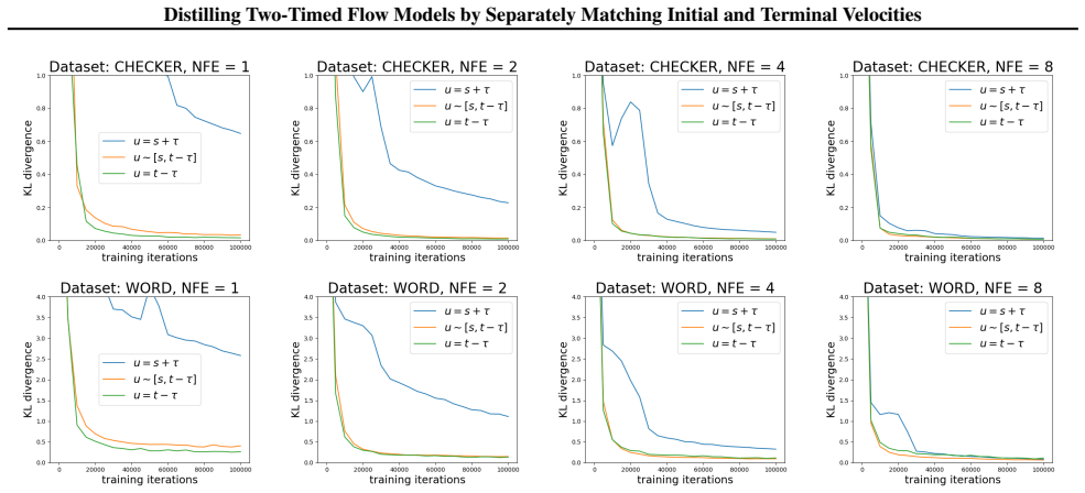
- [Section 5.2, Figures 2 and 3] The conclusions about the intermediate-time choice and step size tau are based on training curves; adding the final metric values and, where applicable, fused ranks would make the claims easier to verify quantitatively.
- [Throughout] There are several typographical and spacing artifacts, including 'V elocities' in the title and inconsistent spacing in 'LIA VM' and 'IA VM'; these should be cleaned up before publication.
Circularity Check
No significant circularity: the proposed loss is a constructive design whose conditional characterization theorem follows from the loss definitions, and the empirical claims are not derived from fitted constants.
full rationale
The paper's central derivation is a constructive loss-design argument followed by a conditional characterization theorem. Theorem 4.3 states that if training drives L_ITVM to zero with the EMA at steady state, then the trained TTFM satisfies phi_theta_{m tau, n tau}(x) = S^eta,tau_{m tau, n tau}(x); this is proved directly from the definitions of the loss terms: L_TVM = 0 yields the consistency relation (5), and L_IAVM = 0 yields the short-interval base case (6), after which the chain over grid points is immediate. The conclusion is a logical consequence of the stated sufficient condition, not an input assumed as the conclusion. The initial velocity terms anchor the loss to the pretrained teacher, and the TVM term's EMA target is explicitly described as a self-consistency objective rather than an independent source of the theorem. The reported experiments compare ITVM against baselines; the main tables select the best ITVM EMA decay via reciprocal rank fusion on test metrics, which is a methodological weakness concerning hyperparameter selection, but it does not make the measured outcome equal to the loss by construction. The only self-citation (Preechakul et al. 2022 for the MLPSkipNet architecture used in tabular experiments) is not load-bearing for the claimed derivation. No equation in the paper reduces to a fitted parameter renamed as a prediction, and no load-bearing claim is justified solely by a self-citation chain.
Assumptions & free parameters
free parameters (3)
- tau (ITVM step size) =
0.005
- EMA decay rate mu =
0, 0.9, 0.99, or 0.999 per dataset
- sigma_min =
0.001
assumptions (4)
- domain assumption The student flow map phi_theta_{s,t} is a diffeomorphism for each (s,t) used in evaluation.
- domain assumption The one-step ODE solver S^eta,tau is a sufficiently accurate approximation of the true teacher flow over intervals of length tau.
- standard math p_s has full support on R^d for all s (Gaussian noise with sigma_min > 0).
- standard math Continuity of v_theta, v_eta, phi_theta, and S^eta,tau.
Cite this review
Pith. "Pith review of Distilling Two-Timed Flow Models by Separately Matching Initial and Terminal Velocities." pith.science (2026). https://pith.science/paper/EQEGIYZ5
@misc{pith2026250501169,
  author       = {Pith},
  title        = {Pith review of: Distilling Two-Timed Flow Models by Separately Matching Initial and Terminal Velocities},
  year         = {2026},
  howpublished = {\url{https://pith.science/paper/EQEGIYZ5}},
  note         = {Machine review of arXiv:2505.01169}
}
abstract
A flow matching model learns a time-dependent vector field $v_t(x)$ that generates a probability path $\{ p_t \}_{0 \leq t \leq 1}$ that interpolates between a well-known noise distribution ($p_0$) and the data distribution ($p_1$). It can be distilled into a two-timed flow model (TTFM) $\phi_{s,x}(t)$ that can transform a sample belonging to the distribution at an initial time $s$ to another belonging to the distribution at a terminal time $t$ in one function evaluation. We present a new loss function for TTFM distillation called the \emph{initial/terminal velocity matching} (ITVM) loss that extends the Lagrangian Flow Map Distillation (LFMD) loss proposed by Boffi et al. by adding redundant terms to match the initial velocities at time $s$, removing the derivative from the terminal velocity term at time $t$, and using a version of the model under training, stabilized by exponential moving averaging (EMA), to compute the target terminal average velocity. Preliminary experiments show that our loss leads to better few-step generation performance on multiple types of datasets and model architectures over baselines.
Figures


Figures from the paper (6 more)



Reference graph
Works this paper leans on
-
[1]
The closer the student distributions are to the teacher distribution, the better the student performs. A well-known way to measure the difference between two probability distributions is the Kullback–Leibler (KL) divergence. Given two probability distributionsp andq over the same domain, the KL divergence ofp with respect toq is defined as KLpp}qq“ Ex„p „...
work page 2020
-
[2]
We denote the push-forward withrφs˚p
Compute φpxq and return the result. We denote the push-forward withrφs˚p. It is well-known that, qpyq“ ` rφs˚p ˘ pxq“ ppφ´1pyqq | det ∇φpφ´1pyqq| (7) for anyyP Rd. Here, ∇φpxq denotes the Jacobian matrix ofφ at pointx. B.1.2. P ROBLEM SETUP Recall from Section 3, we want to model a probability pathtpt :tPr 0, 1su. To do so, We first train a flow matching ...
-
[3]
Here,τ is a small constant, which is fixed to 0.005
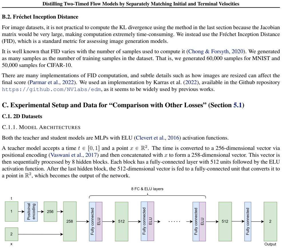
Choosing u“t´τ, which is employed by our proposed TVM. Here,τ is a small constant, which is fixed to 0.005. When implementing the second strategy, we set the upper limit ofu to t´τ instead oft to prevent the denominatort´u on the RHS of (10) to be too small. The EMA decay rate µ was fixed to 0.99. For each of the CHECKER and WORD datasets, we trained 3 st...
-
[4]
URL http://jmlr.org/papers/v15/ srivastava14a.html. Tee, J. T. J., Zhang, K., Yoon, H. S., Gowda, D. N., Kim, C., and Yoo, C. D. Physics informed distillation for diffusion models, 2024. URL https://arxiv.org/ abs/2411.08378. Vaswani, A., Shazeer, N., Parmar, N., Uszkoreit, J., Jones, L., Gomez, A. N., Kaiser, L. u., and Polosukhin, I. Attention is all yo...
arXiv 2024
-
[5]
cc/paper_files/paper/2017/file/ 3f5ee243547dee91fbd053c1c4a845aa-Paper
URL https://proceedings.neurips. cc/paper_files/paper/2017/file/ 3f5ee243547dee91fbd053c1c4a845aa-Paper. pdf. Xie, S., Xiao, Z., Kingma, D. P., Hou, T., Wu, Y . N., Murphy, K. P., Salimans, T., Poole, B., and Gao, R. EM distillation for one-step diffusion models, 2024. URL https:// arxiv.org/abs/2405.16852. Yin, T., Gharbi, M., Park, T., Zhang, R., Shecht...
arXiv 2017
-
[8]
The teacher uses dropout (Srivastava et al., 2014) layers with probability 0.2, but the student does not. We tried a student architecture with such layers, but we found that samples quality degraded significantly
work page 2014
-
[9]
Again, the teacher takes only one time variablet as input, but the student takes 2. In the teacher,t is converted to a 1024- dimensional vector via positional encoding, which is then processed by a 2-layered MLP to yield a 1024-dimensional conditioning vector. This conditioning vector is used to condition all ResNet (He et al., 2016) blocks inside the net...
work page 2016
-
[10]
Choosing u“s`τ, which is employed by CM
Show all 12 references
-
[11]
Sampling u„ Urs,ts, which is employed by SCM
-
[45]
Rezende, D
URL https://www.sciencedirect.com/ science/article/pii/S0021999118307125. Rezende, D. J. and Mohamed, S. Variational inference with normalizing flows, 2016. URL https://arxiv. org/abs/1505.05770. Salimans, T. and Ho, J. Progressive Distillation for Fast Sampling of Diffusion M...
2016 arXiv
-
[2014]
cc/paper_files/paper/2014/file/ 5ca3e9b122f61f8f06494c97b1afccf3-Paper
URL https://proceedings.neurips. cc/paper_files/paper/2014/file/ 5ca3e9b122f61f8f06494c97b1afccf3-Paper. pdf. He, K., Zhang, X., Ren, S., and Sun, J. Deep residual learning for image recognition. In 2016 IEEE Conference on Computer Vision and Pattern Recognition (CVPR), pp. 77...
2014 arXiv
-
[2017]
cc/paper_files/paper/2017/file/ 6c1da886822c67822bcf3679d04369fa-Paper
URL https://proceedings.neurips. cc/paper_files/paper/2017/file/ 6c1da886822c67822bcf3679d04369fa-Paper. pdf. Parmar, G., Zhang, R., and Zhu, J.-Y . On aliased resizing and surprising subtleties in GAN evaluation. In CVPR, 2022. Preechakul, K., Chatthee, N., Wizadwongsa, S., a...
2017
Reviewed August 16, 2026 · model on record in the stance chip above.
Discussion (0). Continue with ORCID to comment.