REVIEW 2 major objections 9 minor 1 cited by
Realization of all-to-all fermion propagator for the first principle high accuracy strong interaction prediction
T0 review · 2 major / 9 minor · reviewed 2026-08-16 · deepseek-v4-flash
Pith's one-line read The paper claims that a "blending" of a few low-frequency spatial modes with random high-frequency modes gives an unbiased, low-cost estimator of the all-to-all quark propagator, and demonstrates sub-percent nucleon axial charges and a…
desk verdict Clever, useful blend of distillation and stochastic high modes that checks out for the demonstrated cases, but the arbitrary-N-point claim outruns the proof. read the letter →
The pith
A machine-rendered reading of the paper's core claim, the machinery that carries it, and where it could break.
The reading
What carries the argument
The load-bearing object is the blending space: the span of $N_e$ low-lying eigenvectors of the spatial Laplace operator (the distillation subspace) plus $N_{st}$ orthonormal random vectors sampled uniformly from its orthogonal complement. The identity that carries the argument is Eq. (12), $\mathbb{E}\left[\sum_{i,j=1}^{N_e+N_{st}}\Omega_{ij}\,\lvert\phi_i\rangle\langle\phi_i\rvert\otimes\lvert\phi_j\rangle\langle\phi_j\rvert\right]=\hat{I}\otimes\hat{I}$, with the reweighting factors $\omega_n=([L_2]-n)/(N_{st}-n)$ and $\Omega_{ij}^{(2)}$ given in Eq. (3). The proof fixes the second and fourth moments of the random vectors by unitary invariance, which is exactly what converts the projected operator into an unbiased estimator while keeping the low-mode part exact. This mechanism is what lets hadron states be constructed by distillation and local currents be inserted without bias.
What would settle it
Set $N_{st}$ equal to the full complement dimension $[L_2]$ on a small lattice, compute the pion conserved-charge ratio of Eq. (5) with the blending estimator, and compare it with the exact point-source value at every time slice; exact agreement would confirm Eq. (12), while any $t$-dependent deviation would falsify the unbiasedness claim.
Extended reading notes
Core claim
The central discovery is that the all-to-all fermion propagator does not need to be stored or inverted in full. The paper constructs a blending space from $N_e$ low-lying eigenvectors of the spatial Laplacian and $N_{st}$ random orthonormal vectors in the orthogonal complement, and assigns a reweighting tensor $\Omega_{ij}$ so that the expectation of the projected identity is $\hat{I}\otimes\hat{I}$. This identity means that every quark-bilinear operator $O=\bar q M_O q$ evaluated in the blending space has expectation equal to the exact operator, with the low-mode sector exact and the high-mode sector unbiased. Consequently the all-to-all propagator is compressed from $(4N_cN_TN_L^3)^2$ to $(4N_T(N_e+N_{st}))^2$ degrees of freedom. Numerical checks include the pion conserved charge, the pion form factor from three- and four-point functions, and sub-percent nucleon axial charges from a joint $N_e$-dependent fit.
Load-bearing premise
The $g_A$ extraction assumes that two effective excited states, one near the nucleon-pion threshold and one near 1.4 GeV, whose masses and $N_e$-dependent weights are fitted to the same data, capture all excited-state contamination in the chosen fit ranges.
Editorial extensions
If this is right
- Any quark-bilinear current, including disconnected quark loops and four-point currents, can be evaluated from the same projected propagators instead of new sequential inversions.
- The compression of the all-to-all propagator from $(4N_cN_TN_L^3)^2$ to $(4N_T(N_e+N_{st}))^2$ degrees of freedom makes large spatial volumes and small lattice spacings comparatively cheaper than in standard all-to-all approaches.
- Varying $N_e$ changes the smearing of the external hadron, so excited-state contamination can be mapped out systematically; the joint three-state fit gives $g_A^{u-d}=1.2339(43)$ with 40 configurations at $m_\pi\simeq300$ MeV.
- The consistency of three- and four-point pion form factors demonstrates that $N$-point correlation functions with two current insertions are practical, opening a route to QED corrections and hadronic-tensor calculations.
Reading between the lines
- If the unbiasedness identity holds at finite $N_{st}$ with the quoted scaling, the same blending-space propagators can be reused for many operators and momenta, so the marginal cost of a new $N$-point observable should become a contraction cost rather than new fermion inversions, an economy the paper only partially exploits.
- The effective second excited state at $\Delta_2\simeq1.42$ GeV is likely a mixture of single-particle and multiparticle states; a GEVP analysis with $\pi N$ and $\pi\pi N$ interpolators on the same blending-space propagators would show whether the three-state model has hidden state-dependent bias in $g_A$.
- The paper notes a difference between its coarse and fine ensemble results for $g_A^{u-d}$; a dedicated continuum-extrapolation study would determine how much of that gap is discretization error versus finite-volume effects.
Signed reviews
Editorial analysis
A structured set of objections, weighed in public.
Referee Report
Summary. The paper introduces the 'blending' method for estimating all-to-all fermion propagators in lattice QCD. At each time slice, the spatial Dirac-color-site space L is split into a low-mode subspace L1 spanned by Ne eigenvectors of the Laplace operator and its complement L2, and the identity on L is represented in expectation by the Ne exact low modes plus Nst random vectors sampled from L2, with reweighting factors ωn = ([L2]−n)/(Nst−n). Propagators projected onto this blending space compress the all-to-all propagator from (4NcNTN_L^3)^2 to (4NT(Ne+Nst))^2 degrees of freedom, and quark-bilinear operators are reweighted to be unbiased in expectation; the supplement proves this single-bilinear unbiasedness (Eq. 12) using the Haar-random moments of the noise vectors. Numerical anchors include: the pion conserved vector charge R_V^π = 1.0002(29) on C24P29; pion form factors from 3-point and 4-point functions that agree (charge radii 0.332(29) and 0.329(33) fm^2); RI/MOM Z_q from the blended propagators matching the point-source result; and, on F48P30 (a = 0.077 fm, mπ ≈ 300 MeV, 40 configurations), a joint 3-state fit over eight Ne values giving g_A^{u−d} = 1.2339(43) and flavor-decomposed g_A^u = 0.895(15), g_A^d = −0.338(15), g_A^s = −0.0245(72), g_A^{u+d+s} = 0.533(28). The authors argue the method makes disconnected diagrams, excited-state control with distillation-like smearing, and N-point functions (QED/isospin corrections, hadronic tensors) practical.
Significance. Assuming the central claim survives, this is a significant methodological contribution: it restores the high-frequency spatial modes that distillation discards, in an unbiased stochastic way, while retaining distillation's excited-state control and multi-operator flexibility; if it generalizes as claimed, it makes disconnected and multi-current correlators with excited-state systematics tractable on large volumes. The strengths are concrete: the unbiasedness proof for a single bilinear is an explicit moment construction (Supplemental Eqs. 12–23), not a fitted result; the numerical anchors are independent and quantitative (conserved vector charge 1.0002(29); RI/MOM Z_q matching point-source propagators in Supp. Fig. 9; 3pt/4pt form-factor agreement); and g_A^{u−d} = 1.2339(43) agrees with high-statistics external determinations (RQCD 1.238(24), CalLAT 1.235(11)), which is nontrivial evidence that the estimator is not tuned to its own constants. The scaling claims (statistical advantage ∝ N_L^{−3/2}, noise saturation at Nst ~ 100–400) are supported by the tests shown.
major comments (2)
- [Supplemental Sec. A.1, Eqs. (12), (21), (25); Abstract/Introduction/Summary] The claim that the method enables 'arbitrary-point correlation functions' is not established for multiple quark-bilinear insertions that share a time slice. The proof in Supplemental Sec. A.1 establishes only the two-leg unbiasedness of Eq. (12) for a single kernel, and the fourth-moment factorization in Eq. (25) is valid only for independent time slices. For two insertions at the same time slice, the estimator is a product of two sums over the same Nst random vectors, and its expectation requires contracting the same-time fourth moments of Eq. (21) with the product of two Ω^(2) weight tensors, a computation the paper does not perform; the sentence 'The proof for more non-trivial cases can be obtained using the similar procedure' is therefore not justified. A minimal check isolates the problem: for Ne = 0, D = 2, Nst = 1, the single-current estimator Ĵ(x) = ω0|η(x)|^2 with ω0 = 2 is unbiased (E[Ĵ] = 1), but E[Ĵ(x)Ĵ(y)] = 4E[|η(x)|^2|η(y)|^2] = 4/(D(D+1)) = 2/3 ≠ 1 for x ≠ y. The demonstrated applications are not affected — the 4pt pion form factor uses t2 − t1 ≥ 2a, and the RI/MOM Z_q check in Fig. 9 validates the three-leg weight Ω^(3) empirically — so the required repair is either a proof for coincident insertions (e.g., a four-leg analogue of Eq. (12) with a weight tensor that is not the product of two Ω^(2) factors) or an explicit restriction of the claim to insertions on distinct time slices.
- [Sec. C.2, Eqs. (49)–(50), Table IV] The headline results (g_A^{u−d} = 1.2339(43), g_A^u = 0.895(15), g_A^d = −0.338(15), g_A^s = −0.0245(72), g_A^{u+d+s} = 0.533(28)) are quoted with jackknife statistical errors only. The 3-state ansatz of Eqs. (49)–(50) represents the entire excited-state contamination by two effective states with Δ1 ≈ 0.49 GeV and Δ2 ≈ 1.4 GeV, and the fit parameter c11 = −0.08(53) is effectively unconstrained; no variation of the number of states, fit ranges, or the set of Ne values is reported to bound the resulting systematic uncertainty. Moreover, the C24P29 ensemble at a = 0.105 fm yields g_A^{u−d} = 1.1690(72), about 5% lower than the F48P30 result, an offset the paper attributes to 'discretization errors and finite volume effects' without quantifying it. For claims such as 'sub-percent determinations' and 'first principle high accuracy' in the title, Introduction, and Abstract, the paper needs a systematic error budget (fit-ansatz variation, renormalization-scale uncertainty from Z_s,MS_A/Z_V = 1.115(15), and an explicit statement that the result is a single-lattice-spacing, fixed-pion-mass demonstration), or the claims must be scoped accordingly.
minor comments (9)
- [Main text Eq. (8)] The excited-state term appears as 'ci0di(e^{−Δi(tf−t)} + e^{−Δi t}) ciid^2_i e^{−Δi tf}', which is missing the '+' before the cii term; compare with the correct form in Supplemental Eq. (49).
- [Main text Eq. (1)] The definition 'ωn = ([L2]−n)/)/(Nst−n)' contains a stray '/)' and should read (([L2]−n)/(Nst−n)); the superscripts on Ω (Ω^(1), Ω^(2)) are also used before being defined.
- [Abstract] The LaTeX '{\color{black} ...}' markup around the g_A values should be removed before submission.
- [Supplemental Eq. (37) and Eq. (36)] The conditions defining Ω^(3) are incomplete: 'i≠j≠k>Ne' does not specify whether the indices are pairwise distinct, and 'all the permutation of i,j,k' does not enumerate the weights for mixed cases such as i=j>Ne with k≤Ne; additionally, 'Ω(2)ij/V' in Eq. (36) contains a dangling '/V'.
- [Fig. 13 and Sec. C.2] The text refers to 'Ne = 80 (left lower panel)', but the panels are labeled Ne = 40, 55, 70, 100; the text should match the figure labels.
- [Sec. C.2] The two-state fit at the 'optimal' Ne value is reported to give exactly g_A^{u−d} = 1.2339(43), the same value as the three-state joint fit; please clarify whether this is an independent fit and how its uncertainty was obtained.
- [Main text references] The generic reference to 'Supplemental materials [33]' in the main text should be replaced by pointers to the specific supplement sections (A.1, A.4, B, C) and equation numbers.
- [Supplemental Sec. A.5] The sentence 'the statistical uncertainty of ⟨V4^cc⟩π scales approximately as Nst^{−1}, as the expectation value of RVπ is exactly one' conflates the mean and the variance of the ratio; please rephrase (the ratio's expectation value is exactly one, and its variance is what scales as Nst^{−2} for the quoted Nst^{−1} uncertainty).
- [Supplemental Eqs. (10)–(13)] The floor notation '⌊L2⌋' is used for the dimension of L2, which is already an exact integer [L2] = NcN_L^3 − Ne; please use [L2] consistently.
Circularity Check
No significant circularity: the blending estimator is a direct moment construction and physics results are externally benchmarked; flagged items are an omitted proof and a non-load-bearing self-citation, not circular reductions.
full rationale
The derivation chain is not circular. The blending estimator's unbiasedness (Eqs. 1-3, 12-24) is a direct moment construction: the weights omega_n are fixed by the noise probability density, and the fourth-moment identities in Eq. (21) are solved from unitary invariance plus normalization/orthogonality constraints, not from the target expectation. Independent checks anchor the construction: the conserved-current ratio gives 1.0002(29) (Fig. 1), the pion dispersion relation is consistent with the continuum, and the pion charge radius from 3pt/4pt agrees with an external chiQCD result. The g_A values are extracted by standard spectral fits (Eqs. 49-50); the three-state ansatz is fitted to the lattice data, not an input that forces the result, and the numbers agree with external RQCD and CalLAT calculations. The singlet renormalization factor Z_s^A/Z_ns^A = 1.054(14) is a self-citation (Ref. [2], co-authored by Y.-B. Yang), but it is an independent published lattice input used only at the renormalization stage, not the basis of the blending method, and it is externally falsifiable. The supplement's statement that 'the proof for more non-trivial cases can be obtained using the similar procedure' is an omitted proof for same-time multi-current insertions and is a completeness/correctness concern, not a circular reduction; the demonstrated applications with currents at different time slices rely on the independent-time-slice factorization of Eq. (25). No step reduces a prediction to a fitted parameter or to a self-citation chain.
Assumptions & free parameters
free parameters (4)
- Ne, Nst subspace sizes =
Ne=100, Nst=200 (F48P30); Ne=100, Nst=400 (C24P29)
- 3-state fit parameters Z(Ne), d1(Ne), d2(Ne), Delta1, Delta2, c10, c20, c11, c21, c22, m0 =
Tables IV-VI; gA^u-d c00=1.2339(43), Delta1=0.493(27), Delta2=1.420(74) GeV
- Renormalization constants Zns_A/ZV and Zs_MS(2 GeV)/ZV =
1.05794(29) and 1.115(15)
- z-expansion coefficients a0, a1, a2 for f_pi(Q^2) =
a0 ~ 0.783, a1 ~ -2.15, a2 ~ 3.3
assumptions (5)
- domain assumption Euclidean lattice QCD with Nf=2+1 dynamical quarks is the correct nonperturbative definition of QCD for these observables.
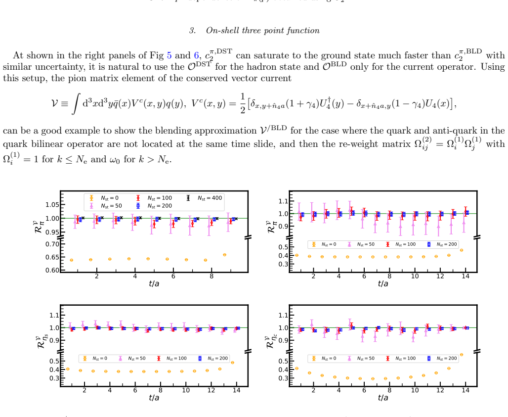
- domain assumption Low-lying eigenvectors of the stout-smeared discrete Laplace operator form a subspace that supports hadron interpolation fields with controlled excited-state overlap.
- standard math The random vectors sampled from L2, after deflation and Gram-Schmidt, have a unitary-invariant joint distribution with the fourth moments in Eq. (21).
- ad hoc to paper The 3-state fit in Eqs. (49)-(50) with two effective excited states fully describes the excited-state contamination over the chosen t and tf ranges.
- domain assumption The singlet renormalization factor Zs_A/Zns_A=1.054(14) from Ref. [2] and the perturbative matching Eq. (39) are valid for this lattice action and scale.
Cite this review
Pith. "Pith review of Realization of all-to-all fermion propagator for the first principle high accuracy strong interaction prediction." pith.science (2026). https://pith.science/paper/6VDGLF36
@misc{pith2026250501719,
  author       = {Pith},
  title        = {Pith review of: Realization of all-to-all fermion propagator for the first principle high accuracy strong interaction prediction},
  year         = {2026},
  howpublished = {\url{https://pith.science/paper/6VDGLF36}},
  note         = {Machine review of arXiv:2505.01719}
}
abstract
We propose a ``blending" algorithm that projects the all-to-all fermion propagator onto spatial low-frequency modes (LFM) combined with a stochastic estimate of spatial high-frequency modes (SHFM) at each time slice. This approach enables the calculation of arbitrary-point correlation functions for arbitrary hadron states in strongly interacting quantum field theories (QFT) with fermions, such as quantum chromodynamics (QCD). Specifically, LFM allows the construction of spatially extended hadron states below a certain energy threshold by diagonalizing multi-fermion interpolation fields. Meanwhile, the local interactions required for N-point correlation functions in QFT can be approximated in an unbiased manner through a reweighted summation of both LFM and SHFM contributions. To demonstrate the efficiency of this algorithm, we obtained {\color{black} $g_A^u=0.895(15)$, $g_A^d=-0.338(15)$, $g_A^s=-0.0245(72)$, $g_A^{u+d+s}=0.533(28)$ and $g_A^{u-d}=1.2339(43)$ } for nucleon at $m_{\pi}=300$ MeV and $a=0.077$ fm using 40 configurations. The consistency check of the pion electric form factor and charge radius derived from 3-point and 4-point correlation functions is also provided.
Figures


Figures from the paper (12 more)




Forward citations
Cited by 1 Pith paper
-
Pion Transition Form Factor in Lattice QCD
The disconnected quark-loop contribution to the pion transition form factor has the same sign as the connected contribution, at roughly 1% of its size, as calculated on one N_f=2+1 clover ensemble.
Reference graph
Works this paper leans on
-
[1]
Subspace L1 (that used in the distillation method [23]): The span of the Ne low-lying eigenvectors {vλi}Ne i=1 of the discrete Laplace operator
-
[2]
Complement subspace L2: The orthogonal com- plement of L1 inL, i.e., L2 = L/L1, with dimension [L2] =NcN3 L−Ne. A “blending space” is constructed by combining the eigenvectors{ϕi ≡ vλi}Ne i=1 spanningL1, and a set of Nst orthogonal random vectors{ϕNe+j≡ηj}Nst j=1 sampled uniformly from L2. Then the identity operator ˆI onL can be unbiasedly approximated a...
-
[3]
Y. Aoki et al. (Flavour Lattice Averaging Group (FLAG)), (2024), arXiv:2411.04268 [hep-lat]
arXiv 2024
-
[4]
J. Liang, Y.-B. Yang, T. Draper, M. Gong, and K.-F. Liu, Phys. Rev. D 98, 074505 (2018), arXiv:1806.08366 [hep-ph]
arXiv 2018
-
[5]
S. Park, R. Gupta, B. Yoon, S. Mondal, T. Bhattacharya, Y.-C. Jang, B. Jo´ o, and F. Winter (Nucleon Matrix Elements (NME)), Phys. Rev. D 105, 054505 (2022), arXiv:2103.05599 [hep-lat]
arXiv 2022
-
[6]
R. E. Smail et al. (QCDSF/UKQCD/CSSM), Phys. Rev. D 108, 094511 (2023), arXiv:2304.02866 [hep-lat]
arXiv 2023
-
[7]
G. S. Bali, S. Collins, S. Heybrock, M. L¨ offler, R. R¨ odl, W. S¨ oldner, and S. Weish¨ aupl (RQCD), Phys. Rev. D 108, 034512 (2023), arXiv:2305.04717 [hep-lat]
arXiv 2023
-
[8]
D. Djukanovic, G. von Hippel, H. B. Meyer, K. Ot- tnad, and H. Wittig, Phys. Rev. D 109, 074507 (2024), arXiv:2402.03024 [hep-lat]
arXiv 2024
Show all 70 references
-
[9]
Chang, A
C.-C. Chang, A. N. Nicholson, E. Rinaldi, E. Berkowitz, N. Garron, D. A. Brantley, H. Monge-Camacho, C. J. Monahan, C. Bouchard, M. A. Clark, et al., Nature 558, 91 (2018)
2018
-
[10]
Walker-Loud et al
A. Walker-Loud et al. , PoS CD2018, 020 (2020), arXiv:1912.08321 [hep-lat]
2020 arXiv
-
[11]
Y.-C. Jang, R. Gupta, T. Bhattacharya, B. Yoon, and H.-W. Lin (Precision Neutron Decay Matrix Ele- ments (PNDME)), Phys. Rev. D 109, 014503 (2024), arXiv:2305.11330 [hep-lat]
2024 arXiv
-
[12]
Alexandrou, S
C. Alexandrou, S. Bacchio, M. Constantinou, J. Finken- rath, R. Frezzotti, B. Kostrzewa, G. Koutsou, G. Spanoudes, and C. Urbach (Extended Twisted Mass), Phys. Rev. D109, 034503 (2024), arXiv:2309.05774 [hep- lat]
2024 arXiv
-
[13]
P. D. G. et.al, Progress of Theoretical and Experimental Physics 2020, 083C01 (2020), https://academic.oup.com/ptep/article- pdf/2020/8/083C01/34673722/ptaa104.pdf
2020
-
[14]
Cirigliano, J
V. Cirigliano, J. de Vries, L. Hayen, E. Mereghetti, and A. Walker-Loud, Phys. Rev. Lett. 129, 121801 (2022)
2022
-
[15]
Borsanyi et al
S. Borsanyi et al. (BMW), Science 347, 1452 (2015), arXiv:1406.4088 [hep-lat]. 6
2015 arXiv
-
[16]
Giusti, V
D. Giusti, V. Lubicz, C. Tarantino, G. Martinelli, F. San- filippo, S. Simula, and N. Tantalo, Phys. Rev. D 95, 114504 (2017), arXiv:1704.06561 [hep-lat]
2017 arXiv
- [17]
-
[18]
C. W. Bernard, T. Draper, G. Hockney, A. M. Rushton, and A. Soni, Phys. Rev. Lett. 55, 2770 (1985)
1985
-
[19]
Y.-B. Yang, A. Alexandru, T. Draper, M. Gong, and K.- F. Liu, Phys. Rev. D93, 034503 (2016), arXiv:1509.04616 [hep-lat]
2016 arXiv
- [20]
-
[21]
Li, S.-C
Y. Li, S.-C. Xia, X. Feng, L.-C. Jin, and C. Liu, Phys. Rev. D 103, 014514 (2021), arXiv:2009.01029 [hep-lat]
2021 arXiv
-
[22]
P.-X. Ma, X. Feng, M. Gorchtein, L.-C. Jin, K.-F. Liu, C.-Y. Seng, B.-G. Wang, and Z.-L. Zhang, Phys. Rev. Lett. 132, 191901 (2024), arXiv:2308.16755 [hep-lat]
2024 arXiv
-
[23]
Gong et al
M. Gong et al. (XQCD), Phys. Rev. D88, 014503 (2013), arXiv:1304.1194 [hep-ph]
2013 arXiv
-
[24]
Giusti, T
L. Giusti, T. Harris, A. Nada, and S. Schaefer, Eur. Phys. J. C 79, 586 (2019), arXiv:1903.10447 [hep-lat]
2019 arXiv
-
[25]
Peardon, J
M. Peardon, J. Bulava, J. Foley, C. Morningstar, J. Dudek, R. G. Edwards, B. Jo´ o, H.-W. Lin, D. G. Richards, and K. J. Juge (Hadron Spectrum Collabo- ration), Phys. Rev. D 80, 054506 (2009)
2009
-
[26]
Morningstar, J
C. Morningstar, J. Bulava, J. Foley, K. J. Juge, D. Lenkner, M. Peardon, and C. H. Wong, Physical Re- view D—Particles, Fields, Gravitation, and Cosmology 83, 114505 (2011)
2011
-
[27]
R. G. Edwards, J. J. Dudek, D. G. Richards, and S. J. Wallace, Phys. Rev. D 84, 074508 (2011), arXiv:1104.5152 [hep-ph]
2011 arXiv
-
[28]
J. J. Dudek, R. G. Edwards, and C. E. Thomas (Hadron Spectrum), Phys. Rev. D 87, 034505 (2013), [Erratum: Phys.Rev.D 90, 099902 (2014)], arXiv:1212.0830 [hep- ph]
2013 arXiv
-
[29]
H. Yan, M. Mai, M. Garofalo, U.-G. Meißner, C. Liu, L. Liu, and C. Urbach, Phys. Rev. Lett. 133, 211906 (2024), arXiv:2407.16659 [hep-lat]
2024 arXiv
- [30]
-
[31]
Wang, Z.-L
X.-H. Wang, Z.-L. Zhang, X.-H. Cao, C.-L. Fan, X. Feng, Y.-S. Gao, L.-C. Jin, and C. Liu, Phys. Rev. Lett. 133, 141901 (2024), arXiv:2310.01168 [hep-lat]
2024 arXiv
-
[32]
Alexandrou, G
C. Alexandrou, G. Koutsou, Y. Li, M. Petschlies, and F. Pittler, PoS LATTICE2024, 317 (2025), arXiv:2412.07263 [hep-lat]
2025 arXiv
-
[33]
Barca, G
L. Barca, G. Bali, and S. Collins, Phys. Rev. D 111, L031505 (2025), arXiv:2412.13138 [hep-lat]
2025 arXiv
-
[34]
Hu et al
Z.-C. Hu et al. (CLQCD), Phys. Rev. D 109, 054507 (2024), arXiv:2310.00814 [hep-lat]
2024 arXiv
-
[35]
Supplemental materials
-
[36]
Du et al
H.-Y. Du et al. (CLQCD), Phys. Rev. D 111, 054504 (2025), arXiv:2408.03548 [hep-lat]
2025 arXiv
-
[37]
R. J. Hill and G. Paz, Phys. Rev. D 82, 113005 (2010)
2010
-
[38]
G. Wang, J. Liang, T. Draper, K.-F. Liu, and Y.- B. Yang (chiQCD), Phys. Rev. D 104, 074502 (2021), arXiv:2006.05431 [hep-ph]
2021 arXiv
- [39]
-
[40]
M. T. Hansen and H. B. Meyer, Nucl. Phys. B 923, 558 (2017), arXiv:1610.03843 [hep-lat]
2017 arXiv
-
[41]
Dalla Brida, T
M. Dalla Brida, T. Korzec, S. Sint, and P. Vilaseca, Eur. Phys. J. C 79, 23 (2019), arXiv:1808.09236 [hep-lat]
2019 arXiv
-
[42]
H.-W. Lin, R. Gupta, B. Yoon, Y.-C. Jang, and T. Bhattacharya, Phys. Rev. D 98, 094512 (2018), arXiv:1806.10604 [hep-lat]
2018 arXiv
-
[43]
Alexandrou, S
C. Alexandrou, S. Bacchio, M. Constantinou, J. Finken- rath, K. Hadjiyiannakou, K. Jansen, G. Koutsou, and A. Vaquero Aviles-Casco, Phys. Rev. D 102, 054517 (2020), arXiv:1909.00485 [hep-lat]
2020 arXiv
-
[44]
Chiu, Phys
T.-W. Chiu, Phys. Rev. D60, 034503 (1999), arXiv:hep- lat/9810052 [hep-lat]
1999
- [45]
- [46]
-
[47]
Ji, Y.-S
X. Ji, Y.-S. Liu, Y. Liu, J.-H. Zhang, and Y. Zhao, Rev. Mod. Phys. 93, 035005 (2021), arXiv:2004.03543 [hep- ph]
2021 arXiv
-
[48]
Ma and J.-W
Y.-Q. Ma and J.-W. Qiu, Phys. Rev. Lett. 120, 022003 (2018), arXiv:1709.03018 [hep-ph]
2018 arXiv
-
[49]
Liu and S.-J
K.-F. Liu and S.-J. Dong, Phys. Rev. Lett. 72, 1790 (1994), arXiv:hep-ph/9306299
1994 arXiv
-
[50]
Liu, Phys
K.-F. Liu, Phys. Rev. D 62, 074501 (2000), arXiv:hep- ph/9910306
2000
-
[51]
Liang, T
J. Liang, T. Draper, K.-F. Liu, A. Rothkopf, and Y.- B. Yang (XQCD), Phys. Rev. D 101, 114503 (2020), arXiv:1906.05312 [hep-ph]
2020 arXiv
-
[52]
Liang, R
J. Liang, R. S. Sufian, B. Wang, T. Draper, T. Khan, K.-F. Liu, and Y.-B. Yang, (2023), arXiv:2311.04206 [hep-lat]
2023 arXiv
-
[53]
Jiang, C
X. Jiang, C. Shi, Y. Chen, M. Gong, and Y.-B. Yang, (2024), arXiv:2411.08461 [hep-lat]
2024 arXiv
-
[54]
M. A. Clark, R. Babich, K. Barros, R. C. Brower, and C. Rebbi, Comput. Phys. Commun. 181, 1517 (2010), arXiv:0911.3191 [hep-lat]
2010 arXiv
-
[55]
Babich, M
R. Babich, M. A. Clark, B. Joo, G. Shi, R. C. Brower, and S. Gottlieb, in SC11 International Conference for High Performance Computing, Networking, Storage and Analysis Seattle, Washington, November 12-18, 2011 (2011) arXiv:1109.2935 [hep-lat]
2011 arXiv
-
[56]
M. A. Clark, B. Jo, A. Strelchenko, M. Cheng, A. Gamb- hir, and R. Brower, (2016), arXiv:1612.07873 [hep-lat]
2016 arXiv
-
[57]
Y.-J. Bi, Y. Xiao, M. Gong, W.-Y. Guo, P. Sun, S. Xu, and Y.-B. Yang, Proceedings, 37th International Sympo- sium on Lattice Field Theory (Lattice 2019): Wuhan, China, June 16-22 2019 , PoS LATTICE2019, 286 (2020), arXiv:2001.05706 [hep-lat]
2020 arXiv
-
[58]
Martinelli, C
G. Martinelli, C. Pittori, C. T. Sachrajda, M. Testa, and A. Vladikas, Nucl. Phys. B445, 81 (1995), arXiv:hep- lat/9411010 [hep-lat]
1995
-
[59]
Bouchard, C
C. Bouchard, C. C. Chang, T. Kurth, K. Orginos, and A. Walker-Loud, Phys. Rev. D 96, 014504 (2017). 7 SUPPLEMENTAL MATERIALS A. Justification of the blending method
2017
-
[60]
blending space
Mathematical Proof For a fixed time slice of a 4D hypercubic lattice of dimensionless size N3 L×NT , we define the space L as the vector space associated with the lattice sites and color degrees of freedom, with dimension [ L] = NcN3 L. Within L, a “blending space” is construc...
-
[61]
Two point function We shall start from the two point function of the point-source and point-sink pion interpolation field π = ¯uγ5d, cπ,PP 2 (⃗ p,t) = Z d3ye−i⃗ y·⃗ p⟨π(⃗ y,t)π†(⃗0, 0)⟩ = Z d3ye−i⃗ y·⃗ ptr h S(⃗ y,t,⃗0, 0)γ5S(⃗0, 0,⃗ y,t)γ5 i , (28) and also that with the proj...
-
[62]
On-shell three point function At shown in the right panels of Fig 5 and 6, cπ,DST 2 can saturate to the ground state much faster than cπ,BLD 2 with similar uncertainty, it is natural to use theODST for the hadron state andOBLD only for the current operator. Using this setup, t...
-
[63]
Off-shell three point function As an even more complicated example of the blending method, we show its application in the RI/MOM renormal- ization. Taking that of the quark self energy under the RI/MOM scheme [56] as example, Zq(µ) =ZV 1 48Tr[⟨S⟩−1(p)⟨GΓ(p)⟩⟨S⟩−1(p)γµ], (35) w...
-
[64]
Uncertainty scaling and saturation Numerical tests confirm the following scaling behavior for statistical uncertainties with respect to Nst, in agreement with theoretical expectations:
-
[65]
For blended quark bilinear operators without momentum transfer or gauge links, and also off-shell blended quark states: δ1∝N−1/2 st
-
[66]
For blended quark bilinear operators involving either momentum transfer or gauge links: δ2∝N−1 st
-
[67]
For the combinations of N objects in case 1 and M objects in case 2: δ∝δN 1 δM 2 . In Fig. 8, we observe that the statistical uncertainty of ⟨Vcc 4 ⟩π scales approximately as N−1 st , as the expectation value of RV π is exactly one. Since the random vectors ηj are sampled inde...
-
[68]
Parameterization By inserting the the complete sets of states, the ratio RO H can be parameterized as: RO H(tf,t ;Ne) = R d3xd3yd3z⟨H(⃗ x,tf)O(⃗ y,t)H†(⃗ z,0)⟩R d3xd3z⟨H(⃗ x,tf)H†(⃗ z,0)⟩ = P iciid2 i (Ne)e−∆itf +P i<jcijdi(Ne)dj(Ne)(e−∆i(tf−t)−∆jt +e−∆j(tf−t)−∆it)P id2 i (Ne)...
-
[69]
13, we present RAu−d N (tf,t ) for various t and tf values, using Ne = 40 (left upper panel), 55 (right upper panel), 80 (left lower panel), and 100 (right lower panel)
3-state fit of gu−d A In Fig. 13, we present RAu−d N (tf,t ) for various t and tf values, using Ne = 40 (left upper panel), 55 (right upper panel), 80 (left lower panel), and 100 (right lower panel). All panels display the same gray bands representing the 18 ground-state matri...
-
[70]
3-state fits of the flavor decomposed gA Our calculations on the F48P30 ensemble reveal that the Ne-dependence of bothRAs N andRAu+d+s N is significantly weaker than expected across various t and tf values, as demonstrated in Fig. 15. These results incorporate the disconnected...
Reviewed August 16, 2026 · model on record in the stance chip above.
Discussion (0). Continue with ORCID to comment.