REVIEW 3 major objections 5 minor 55 references
Heterosynaptic Circuits Are Universal Gradient Machines
T0 review · 3 major / 5 minor · reviewed 2026-08-16 · deepseek-v4-flash
Pith's one-line read This paper argues that gradient learning is the generic outcome of almost any two-signal heterosynaptic plasticity rule, provided the circuit satisfies heterosynaptic stability and dynamical consistency.
desk verdict A genuinely conditional theory of heterosynaptic gradient learning: the algebra is clean, the HSDC framing is new, but the load-bearing HS condition is demonstrated only at a level the universality claim needs. read the letter →
The pith
A machine-rendered reading of the paper's core claim, the machinery that carries it, and where it could break.
The reading
What carries the argument
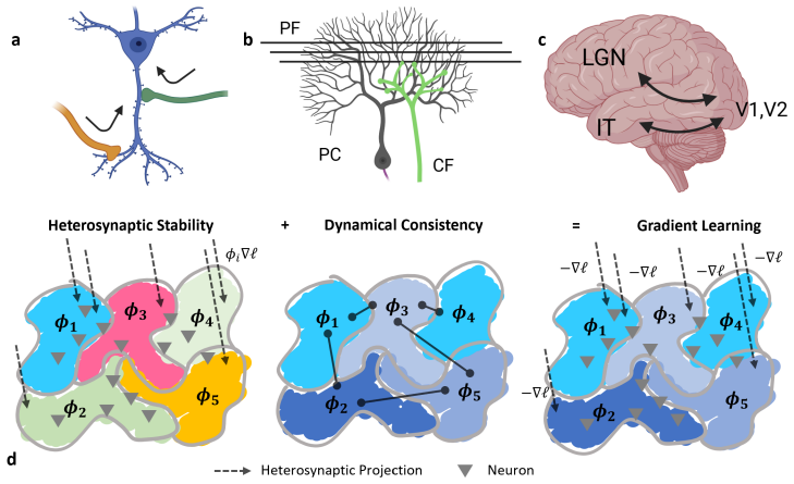
The load-bearing object is the two-signal heterosynaptic update rule, Eq. (2), together with the fixed-point condition on the instructive weight $\bar V$. At $\Delta \bar V = 0$, the stationarity equation $p(t)\bar h(t')^\top = \gamma \bar V$ can be rearranged into $\bar h(t') = \phi \bar V^\top \nabla_p \ell$ with $\phi = \gamma / (\nabla_p^\top \ell\, p)$, and substituting back produces the activation update $p(t') = \phi \bar V \bar V^\top \nabla_p \ell$; the outer product $\bar V \bar V^\top$ therefore plays the role of a plastic matrix learning rate, and the scalar $\phi$, called the consistency score, fixes the sign of learning. Dynamical consistency, $\phi_i \phi_j \ge 0$, is what turns local descent at one node into global descent for the whole circuit. The theorems show that for ReLU-type activations (called radially linear units) consistency holds automatically, and for nondifferentiable activations the same identity holds when the loss is evaluated on a pointwise differentiable approximant.
What would settle it
Train a heterosynaptic circuit of the form in Eq. (2) with random instructive weights $\bar V$, and record for each step the norm $\|\Delta \bar V\|$ together with the cosine alignment between the activation update and the true negative gradient $-\nabla_p \ell$; if alignment is consistently high on steps where $\|\Delta \bar V\|$ is not small, the fixed-point condition is not necessary, while a tight correlation would confirm that heterosynaptic stability is the mechanism.
Extended reading notes
Core claim
On the paper's own terms, the central claim is the HSDC formula: HS + DC = Gradient Learning. For a circuit whose synapses obey the two-signal update $\Delta \bar V = \eta p(t)\bar h(t')^\top - \gamma \bar V$ and $\Delta W = \eta p(t')\bar h(t)^\top - \gamma W$, heterosynaptic stability at a node means the instructive weight is at a fixed point, $\Delta \bar V = 0$; a short rearrangement then gives $\bar h(t') = \phi \bar V^\top \nabla_{p(t)}\ell$, so the receiving neuron's signal is $p(t') = \phi \bar V \bar V^\top \nabla_{p(t)}\ell(p(t))$, which is gradient descent with a positive-semidefinite matrix learning rate $H = \bar V \bar V^\top$ and a scalar consistency score $\phi$. If all consistency scores satisfy $\phi_i \phi_j \ge 0$ for every pair of nodes, every part of the network descends in the same direction, and the chain rule turns this activation gradient into a weight update. The paper concludes that gradient computation is a property of two-signal plasticity near heterosynaptic stability, rather than a property of any particular network architecture or learning algorithm.
Load-bearing premise
The argument assumes that instructive synapses stay near their own stable fixed points while learning happens; if those synapses move substantially during training, the gradient identity in Theorem 1 does not hold.
Editorial extensions
If this is right
- Gradient learning becomes the default of any two-signal circuit that can reach heterosynaptic stability, so biologically plausible learning does not need backpropagation-specific wiring or an explicit error-propagation pathway.
- Observed Hebbian and anti-Hebbian plasticity can be reinterpreted as emergent side effects of heterosynaptic descent: after an update the activation change is proportional to the activation itself, making the rule look Hebbian even when the underlying mechanism is not.
- Because the matrix learning rate $H$ is plastic, such circuits are automatic meta-learners; prior experience changes the effective learning rate of individual synapses, which is the phenomenology of metaplasticity.
- Standard optimizers such as SGD, Adam, RMSProp, and natural gradient are special cases of matrix-learning-rate gradient rules, so the HSDC mechanism places them and biological circuits in one equivalence class.
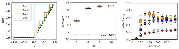
- The circuit can learn through nondifferentiable or low-precision components because only closeness to heterosynaptic stationarity is needed, which allows learning through spiking or quantized activations where plain SGD fails.
Reading between the lines
- A step the paper does not take is proving that the heterosynaptic fixed point is attracting under the update dynamics; if it is, the universality claim extends from stationary inputs to full training trajectories.
- A testable extension for analog hardware is that any physical system with two signal pathways and weight decay that satisfies heterosynaptic stability should implement gradient descent without computing gradients, so one could build a photonic or memristive trainer and measure gradient alignment directly.
- The emergence of dynamical consistency in simulations points to a developmental reading: early dense or random growth followed by pruning may be how a circuit searches over topologies for consistency, with evolution selecting heterosynaptic over Hebbian edges.
Signed reviews
Editorial analysis
A structured set of objections, weighed in public.
Referee Report
Summary. The paper proposes the 'HSDC' design principle: any circuit whose synaptic weights follow a two-signal heterosynaptic update rule of the form (2) implements matrix-learning-rate gradient descent, provided two local conditions hold: Heterosynaptic Stability (HS) and Dynamical Consistency (DC). The formal core is Theorem 1, which shows that at an exact fixed point of the instructive weights, the backward signal satisfies Eq. (7), so the forward update takes the gradient form p(t') = phi Vbar Vbar^T grad_p ell (Eq. (3)); Theorems 3-6 extend the statement to approximate stationarity, nondifferentiable activations, and architectural consistency. Simulations on CIFAR-10 with random connectivity masks, step-ReLU activations, channel rewiring, and an evolutionary growth model are presented as support. The Discussion candidly states that the necessity of HS and the mechanism of DC emergence remain open.
Significance. If the HS condition can be certified for actual learning dynamics, the paper would provide a genuinely unifying statement: feedback alignment, direct feedback alignment, KP, and SAL all become instances of one two-signal motif, and the PSD matrix learning rate connects the result to Adam, RMSProp, and natural gradient. The strengths of the manuscript are its transparent algebraic derivation, its explicit conditional theorem, the breadth of the simulation suite (100 random topologies, step-ReLU, rewiring, evolution), and the falsifiable predictions it generates about metaplasticity, critical periods, and the evolutionary advantage of heterosynaptic plasticity. The central limitation is that the main theorem is conditional on a stationarity assumption that is not proved to hold under the stochastic, nonstationary learning dynamics, so the 'universal' claim in the title is currently stronger than the formal content.
major comments (3)
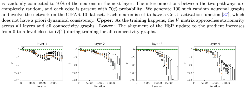
- [C.1, Eq. (12), Theorem 1] The HS condition is a per-input fixed-point condition. Eq. (12) requires p(x) hbar^T(x) = gamma Vbar for each input x to which the theorem is applied. For a fixed matrix Vbar, the left side is rank one, so a single Vbar cannot satisfy this equation for a diverse set of inputs whose p(x) and hbar(x) span more than one direction; at best E_x[p hbar^T] = gamma Vbar can hold. Theorem 1 as stated therefore applies at isolated inputs, not to the learning dynamics over a data set. The aggregate stationarity reported in Figure 9 is an average statement and does not control per-sample deviations, which can be of order Var(p hbar^T)^{1/2}/gamma and need not be small. Because Eq. (3) is the only bridge from the update rule to grad_W ell, the universality claim requires an additional argument showing either that per-sample stationarity is approximately maintained with high probability or that the accumulated error in the weight update is controlled.
- [C.1, Theorem 3 and its Remark] The O(epsilon) relaxation does not resolve the difficulty. If Delta Vbar_i = O(epsilon), the proof of Eq. (28) divides by the scalar grad_{zeta_i}^T ell(F(x,t)) zeta_i(x,t), which need not be bounded away from zero; consequently the O(epsilon) residual in Eq. (33) is not uniformly small. The Remark after Theorem 3 asserts that contributions from other inputs may cancel as noise, but no averaging theorem or variance bound is supplied. Without such a bound, the claim that the actual update dynamics aligns with the gradient is not established.
- [C.2.1, Assumption 1 and Theorem 4] Assumption 1 guarantees only the existence of some c0 > 0 such that c0 Z^T grad_{h1} ell = grad_{h2} ell. The proof of Eq. (40) uses this relation as an equality with no constants, so the exact equalities phi_h = phi_p = phi_{tilde h} are not a logical consequence of the stated assumption. At most equality of signs follows. Since the DC condition (4) requires only sign agreement, this is repairable by restating Theorem 4 as a sign-consistency theorem, but as written the exact equality overreaches, and Theorem 5 inherits the same issue when it compares phi_h Vbar Vbar^T grad_p ell and phi_p W W^T grad_p ell.
minor comments (5)
- [Section 2.2] The statement that the fixed points of the homosynaptic Hebbian update are 'either zero or infinity' is not correct for a fixed input vector: for Delta W = W h h^T - gamma W, nonzero fixed points of the form W = u h^T exist when gamma = ||h||^2. The qualitative point that one fixed matrix cannot serve diverse inputs remains valid, but the supporting sentence should be corrected.
- [Equation (5) and the proof of Theorem 6] The displayed equations contain long corrupted stretches of repeated bracket symbols that are unreadable; these need to be cleaned before publication.
- [Assumption 1] The notation 'Z > 0' is undefined; if it means elementwise positivity, the assumption should be restated in terms of the linear map being invertible or having a well-defined sign, since the proof uses the relation as if Z is an arbitrary matrix satisfying h1 = Z h2.
- [Section 2.4 and Appendix D.6] The claim that delta_hebb and delta_hetero lower-bound the number of Hebbian and heterosynaptic updates relies on an implied causal relation ('if both i and j fired exactly once, then i caused j to fire') that is not established for the recurrent firing rule; please clarify or weaken the interpretation of these metrics.
- [Throughout] There are several typographical errors, including 'Purjinke cells' (should be Purkinje cells), 'thaitn' in the Discussion, and 'cersa' in Figure 5; these should be corrected in a final pass.
Circularity Check
The HS-to-gradient 'theorem' is an algebraic identity at the fixed point, making the central HSDC claim definitional; the evolution experiment additionally selects on loss and reports the resulting gradient alignment as emergence.
-
self definitional
[Appendix C.1, Theorem 1, Eqs. (11)-(14); main text Eq. (3)]
"At stationarity, p¯h⊺ =γ ¯V. (12) Multiplying ∇⊺pℓ from the left, ∇⊺pℓ p¯h⊺ =γ∇⊺pℓ ¯V. (13) Therefore, ¯h=ϕ ¯V⊺∇pℓ. (14)"
Substituting the stationarity equation (12) into (14) gives ¯h = [γ/(pᵀ∇ℓ)] (¯h pᵀ/γ)∇ℓ = ¯h, an identity that holds for any loss ℓ with pᵀ∇ℓ ≠ 0. Thus Eq. (14), and hence the advertised Eq. (3) p(t′) = φH∇_{p(t)}ℓ, contains no information beyond the fixed-point assumption ∆¯V = 0: the 'gradient' direction is unconstrained by ℓ and cancels out. The derivation from HS to gradient learning is therefore a rewrite of the HS definition by construction, not a first-principles derivation.
-
fitted input called prediction
[Section 2.4 / Figure 6 and Appendix D.6 (fitness score definition)]
"The first generation starts from a very sparse activation and evolves according to the fitness score, which is the negative loss function after 100 training steps. The results show interesting results: ... (3) with a dense init., the evolution leads to a steady tendency of sparsification, and gradient learning emerges suddenly as the model becomes sparser."
The fitness is defined as the negative training loss, while the reported outcome is the alignment of the circuit update with the negative loss gradient. For any small update that decreases the loss, the first-order condition ∇ℓ·Δ < 0 gives positive alignment Δ·(−∇ℓ) > 0; hence selecting directly for low loss mechanically selects for positive gradient alignment. The 'gradient learning emerges' claim is therefore substantially forced by the fitness definition rather than an independent test of the HSDC mechanism.
full rationale
The paper's central formal step, Theorem 1 (Appendix C.1), claims that Heterosynaptic Stability (∆¯V = 0) implies ¯h = φ ¯Vᵀ∇pℓ and hence the gradient update p(t′) = φ ¯V ¯Vᵀ∇pℓ. Checking the algebra, this is an exact rewrite of the stationarity condition: substituting p¯hᵀ = γ¯V into the conclusion gives an identity valid for an arbitrary loss function. The conclusion is thus equivalent to the assumption by construction; no property of the learning task enters the direction of the update. This is a self-definitional reduction rather than an empirical or mathematical derivation of gradient learning, and it affects the central HSDC formula, not a peripheral claim. The Remark after Theorem 3 concedes nonstationarity, but the circularity is independent of that concession: even at the exact fixed point, the 'gradient' relation is tautological. A secondary example is the evolution experiment (Sec. 2.4/Fig. 6), where fitness is the negative training loss and the reported 'gradient learning emerges' is the alignment of updates with the negative gradient; since loss-reducing updates are first-order positively aligned with the negative gradient, that result is substantially generated by the fitness choice rather than independently predicted. The paper's self-citations (e.g., SAL [29], representation formation [53]) are used for architectures and context but are not load-bearing for the tautological step; no additional circularity is attributed to them. Because the central derivation reduces by construction to its input fixed-point condition, the appropriate score is high.
Assumptions & free parameters
free parameters (1)
- Root node gain c =
c < 0 (sign unspecified; magnitude not used by theory)
assumptions (6)
- domain assumption Heterosynaptic Stability: for every input used in learning, the instructive weights satisfy ∆Vbar ≈ 0 in Eq. (2).
- ad hoc to paper Two-signal update rule: synaptic weights update as ∆Vbar = η p(t) hbar^T(t') − γ Vbar and ∆W = η p(t') hbar^T(t) − γ W (Eq. 2), or the generalized forms in Eq. (46).
- domain assumption Root node availability: a node computes an error signal hbar = c Vbar^T ∇_{\hat y}ℓ with c < 0.
- domain assumption Path separation implies gradient separation (Assumption 1).
- domain assumption Activations are radially linear (RLU) or pointwise approximable by a smooth network: h = D(p)p with diagonal piecewise-constant D, and nondifferentiable f is approximated by F with ζ_i = p_i + O(ε).
- domain assumption The forward computation graph is acyclic (for Theorem 6).
invented entities (1)
-
Consistency score φ_i
Cite this review
Pith. "Pith review of Heterosynaptic Circuits Are Universal Gradient Machines." pith.science (2026). https://pith.science/paper/WAGYIFGE
@misc{pith2026250502248,
  author       = {Pith},
  title        = {Pith review of: Heterosynaptic Circuits Are Universal Gradient Machines},
  year         = {2026},
  howpublished = {\url{https://pith.science/paper/WAGYIFGE}},
  note         = {Machine review of arXiv:2505.02248}
}
read the original abstract
We propose a design principle for the learning circuits of the biological brain. The principle states that almost any dendritic weights updated via heterosynaptic plasticity can implement a generalized and efficient class of gradient-based meta-learning. The theory suggests that a broad class of biologically plausible learning algorithms, together with the standard machine learning optimizers, can be grounded in heterosynaptic circuit motifs. This principle suggests that the phenomenology of (anti-) Hebbian (HBP) and heterosynaptic plasticity (HSP) may emerge from the same underlying dynamics, thus providing a unifying explanation. It also suggests an alternative perspective of neuroplasticity, where HSP is promoted to the primary learning and memory mechanism, and HBP is an emergent byproduct. We present simulations that show that (a) HSP can explain the metaplasticity of neurons, (b) HSP can explain the flexibility of the biology circuits, and (c) gradient learning can arise quickly from simple evolutionary dynamics that do not compute any explicit gradient. While our primary focus is on biology, the principle also implies a new approach to designing AI training algorithms and physically learnable AI hardware. Conceptually, our result demonstrates that contrary to the common belief, gradient computation may be extremely easy and common in nature.
Figures


Figures from the paper (13 more)




Reference graph
Works this paper leans on
-
[1]
Metaplasticity: tuning synapses and networks for plasticity
Wickliffe C Abraham. Metaplasticity: tuning synapses and networks for plasticity. Nature Reviews Neuroscience, 9(5):387–387, 2008
work page 2008
-
[2]
Deep learning without weight transport
Mohamed Akrout, Collin Wilson, Peter Humphreys, Timothy Lillicrap, and Douglas B Tweed. Deep learning without weight transport. Advances in neural information processing systems , 32, 2019
work page 2019
-
[3]
Natural gradient works efficiently in learning
Shun-Ichi Amari. Natural gradient works efficiently in learning. Neural Comput., 10(2):251–276, Febru- ary 1998
work page 1998
-
[4]
Hebbian plasticity in vivo: relevance and induc- tion
Niels Andersen, Nathalie Krauth, and Sadegh Nabavi. Hebbian plasticity in vivo: relevance and induc- tion. Current opinion in neurobiology , 45:188–192, 2017
work page 2017
-
[5]
Ariana Anderson, Kevin Japardi, Kendra S Knudsen, Susan Y Bookheimer, Dara G Ghahremani, and Robert M Bilder. Big-c creativity in artists and scientists is associated with more random global but less random local fmri functional connectivity. Psychology of Aesthetics, Creativity, and the Arts , 2022
work page 2022
-
[6]
An on-chip photonic deep neural network for image classification
Farshid Ashtiani, Alexander J Geers, and Firooz Aflatouni. An on-chip photonic deep neural network for image classification. Nature, 606(7914):501–506, 2022
work page 2022
-
[7]
Training deep quantum neural networks
Kerstin Beer, Dmytro Bondarenko, Terry Farrelly, Tobias J Osborne, Robert Salzmann, Daniel Scheier- mann, and Ramona Wolf. Training deep quantum neural networks. Nature communications, 11(1):808, 2020
work page 2020
-
[8]
Programmable photonic circuits
Wim Bogaerts, Daniel P´ erez, Jos´ e Capmany, David AB Miller, Joyce Poon, Dirk Englund, Francesco Morichetti, and Andrea Melloni. Programmable photonic circuits. Nature, 586(7828):207–216, 2020
2020
Show all 55 references
-
[9]
Role of feedback connections in central visual processing
Farran Briggs. Role of feedback connections in central visual processing. Annual review of vision science , 6(1):313–334, 2020
2020
-
[10]
Heterosynaptic plasticity prevents runaway synaptic dynamics
Jen-Yung Chen, Peter Lonjers, Christopher Lee, Marina Chistiakova, Maxim Volgushev, and Maxim Bazhenov. Heterosynaptic plasticity prevents runaway synaptic dynamics. Journal of Neuroscience , 33(40):15915–15929, 2013
2013
-
[11]
Heterosynaptic plasticity: multiple mechanisms and multiple roles
Marina Chistiakova, Nicholas M Bannon, Maxim Bazhenov, and Maxim Volgushev. Heterosynaptic plasticity: multiple mechanisms and multiple roles. The Neuroscientist, 20(5):483–498, 2014
2014
-
[12]
Homeostatic role of heterosynaptic plasticity: models and experiments
Marina Chistiakova, Nicholas M Bannon, Jen-Yung Chen, Maxim Bazhenov, and Maxim Volgushev. Homeostatic role of heterosynaptic plasticity: models and experiments. Frontiers in computational neuroscience, 9:89, 2015
2015
-
[13]
On lazy training in differentiable programming
Lenaic Chizat, Edouard Oyallon, and Francis Bach. On lazy training in differentiable programming. arXiv preprint arXiv:1812.07956 , 2018
2018 arXiv
-
[14]
Critical periods of brain development
J Miguel Cisneros-Franco, Patrice Voss, Maryse E Thomas, and Etienne de Villers-Sidani. Critical periods of brain development. In Handbook of clinical neurology , volume 173, pages 75–88. Elsevier, 2020
2020
-
[15]
Measuring the signal-to-noise ratio of a neuron
Gabriela Czanner, Sridevi V Sarma, Demba Ba, Uri T Eden, Wei Wu, Emad Eskandar, Hubert H Lim, Simona Temereanca, Wendy A Suzuki, and Emery N Brown. Measuring the signal-to-noise ratio of a neuron. Proceedings of the National Academy of Sciences , 112(23):7141–7146, 2015
2015
-
[16]
Random noise stimulation improves neuroplas- ticity in perceptual learning
Anna Fertonani, Cornelia Pirulli, and Carlo Miniussi. Random noise stimulation improves neuroplas- ticity in perceptual learning. Journal of Neuroscience , 31(43):15416–15423, 2011. 10
2011
-
[17]
Spike-timing-dependent synaptic plasticity depends on dendritic location
Robert C Froemke, Mu-ming Poo, and Yang Dan. Spike-timing-dependent synaptic plasticity depends on dendritic location. Nature, 434(7030):221–225, 2005
2005
-
[18]
Past makes future: role of pfc in prediction
Joaqu´ ın M Fuster and Steven L Bressler. Past makes future: role of pfc in prediction. Journal of cognitive neuroscience, 27(4):639–654, 2015
2015
-
[19]
Learning and memory impairment in patients with temporal lobe epilepsy: relation to the presence, type, and location of brain lesion
Anna R Giovagnoli and Giuliano Avanzini. Learning and memory impairment in patients with temporal lobe epilepsy: relation to the presence, type, and location of brain lesion. Epilepsia, 40(7):904–911, 1999
1999
-
[20]
Potassium channels control the interaction between active dendritic integration compartments in layer 5 cortical pyramidal neurons
Mark T Harnett, Ning-Long Xu, Jeffrey C Magee, and Stephen R Williams. Potassium channels control the interaction between active dendritic integration compartments in layer 5 cortical pyramidal neurons. Neuron, 79(3):516–529, 2013
2013
-
[21]
The organization of behavior: A neuropsychological theory
Donald Olding Hebb. The organization of behavior: A neuropsychological theory . Psychology press, 2005
2005
-
[22]
Distilling the knowledge in a neural network
Geoffrey Hinton, Oriol Vinyals, and Jeff Dean. Distilling the knowledge in a neural network. arXiv preprint arXiv:1503.02531, 2015
2015 arXiv
-
[23]
State-dependent modulation of sensory feedback
Hans Hultborn. State-dependent modulation of sensory feedback. The Journal of physiology , 533(1):5– 13, 2001
2001
-
[24]
Structural homo-and heterosynaptic plasticity in mature and adult newborn rat hippocampal granule cells
Tassilo Jungenitz, Marcel Beining, Tijana Radic, Thomas Deller, Hermann Cuntz, Peter Jedlicka, and Stephan W Schwarzacher. Structural homo-and heterosynaptic plasticity in mature and adult newborn rat hippocampal granule cells. Proceedings of the National Academy of Sciences ,...
2018
-
[25]
Kingma and Jimmy Ba
Diederik P. Kingma and Jimmy Ba. Adam: A method for stochastic optimization. CoRR, abs/1412.6980, 2014
2014 arXiv
-
[26]
Heb- bian and anti-hebbian spike-timing-dependent plasticity of human cortico-cortical connections
Giacomo Koch, Viviana Ponzo, Francesco Di Lorenzo, Carlo Caltagirone, and Domenica Veniero. Heb- bian and anti-hebbian spike-timing-dependent plasticity of human cortico-cortical connections. Journal of Neuroscience, 33(23):9725–9733, 2013
2013
-
[27]
Principles of plasticity in the developing brain
Bryan Kolb, Allonna Harker, and Robbin Gibb. Principles of plasticity in the developing brain. Devel- opmental Medicine & Child Neurology , 59(12):1218–1223, 2017
2017
-
[28]
Backpropagation without weight transport
John F Kolen and Jordan B Pollack. Backpropagation without weight transport. In Proceedings of 1994 IEEE International Conference on Neural Networks (ICNN’94) , volume 3, pages 1375–1380. IEEE, 1994
1994
-
[29]
Self-assembly of a biologically plausible learning circuit
Qianli Liao, Liu Ziyin, Yulu Gan, Brian Cheung, Mark Harnett, and Tomaso Poggio. Self-assembly of a biologically plausible learning circuit. arXiv preprint arXiv:2412.20018 , 2024
2024 arXiv
-
[30]
Random synaptic feedback weights support error backpropagation for deep learning
Timothy P Lillicrap, Daniel Cownden, Douglas B Tweed, and Colin J Akerman. Random synaptic feedback weights support error backpropagation for deep learning. Nature communications, 7(1):13276, 2016
2016
-
[31]
Backpropa- gation and the brain
Timothy P Lillicrap, Adam Santoro, Luke Marris, Colin J Akerman, and Geoffrey Hinton. Backpropa- gation and the brain. Nature Reviews Neuroscience, 21(6):335–346, 2020
2020
-
[32]
Synaptic plasticity forms and functions
Jeffrey C Magee and Christine Grienberger. Synaptic plasticity forms and functions. Annual review of neuroscience, 43(1):95–117, 2020
2020
-
[33]
Anatomy of hierarchy: feedforward and feedback pathways in macaque visual cortex
Nikola T Markov, Julien Vezoli, Pascal Chameau, Arnaud Falchier, Ren´ e Quilodran, Cyril Huissoud, Camille Lamy, Pierre Misery, Pascale Giroud, Shimon Ullman, et al. Anatomy of hierarchy: feedforward and feedback pathways in macaque visual cortex. Journal of comparative neurol...
2014
-
[34]
Medial prefrontal cell activity signaling prediction errors of action values
Madoka Matsumoto, Kenji Matsumoto, Hiroshi Abe, and Keiji Tanaka. Medial prefrontal cell activity signaling prediction errors of action values. Nature neuroscience, 10(5):647–656, 2007. 11
2007
-
[35]
Direct feedback alignment provides learning in deep neural networks
Arild Nøkland. Direct feedback alignment provides learning in deep neural networks. Advances in neural information processing systems , 29, 2016
2016
-
[36]
Simplified neuron model as a principal component analyzer
Erkki Oja. Simplified neuron model as a principal component analyzer. Journal of mathematical biology , 15:267–273, 1982
1982
-
[37]
Prajit Ramachandran, Barret Zoph, and Quoc V. Le. Searching for activation functions, 2017
2017
-
[38]
Global waves synchronize the brain’s functional systems with fluctuating arousal
Ryan V Raut, Abraham Z Snyder, Anish Mitra, Dov Yellin, Naotaka Fujii, Rafael Malach, and Marcus E Raichle. Global waves synchronize the brain’s functional systems with fluctuating arousal. Science advances, 7(30):eabf2709, 2021
2021
-
[39]
Align, then memorise: the dynamics of learning with feedback alignment
Maria Refinetti, St´ ephane d’Ascoli, Ruben Ohana, and Sebastian Goldt. Align, then memorise: the dynamics of learning with feedback alignment. In International Conference on Machine Learning , pages 8925–8935. PMLR, 2021
2021
-
[40]
A cooperative switch determines the sign of synaptic plasticity in distal dendrites of neocortical pyramidal neurons
Per Jesper Sj¨ ostr¨ om and Michael H¨ ausser. A cooperative switch determines the sign of synaptic plasticity in distal dendrites of neocortical pyramidal neurons. Neuron, 51(2):227–238, 2006
2006
-
[41]
How to train your energy-based models
Yang Song and Diederik P Kingma. How to train your energy-based models. arXiv preprint arXiv:2101.03288, 2021
2021 arXiv
-
[42]
Learning produces an orthogonal- ized state machine in the hippocampus
Weinan Sun, Johan Winnubst, Maanasa Natrajan, Chongxi Lai, Koichiro Kajikawa, Arco Bast, Michalis Michaelos, Rachel Gattoni, Carsen Stringer, Daniel Flickinger, et al. Learning produces an orthogonal- ized state machine in the hippocampus. Nature, pages 1–11, 2025
2025
-
[43]
Tieleman and G
T. Tieleman and G. Hinton. Lecture 6.5—RmsProp: Divide the gradient by a running average of its recent magnitude. COURSERA: Neural Networks for Machine Learning, 2012
2012
-
[44]
Hebb and homeostasis in neuronal plasticity
Gina G Turrigiano and Sacha B Nelson. Hebb and homeostasis in neuronal plasticity. Current opinion in neurobiology, 10(3):358–364, 2000
2000
-
[45]
Homeostatic plasticity in the developing nervous system.Nature reviews neuroscience, 5(2):97–107, 2004
Gina G Turrigiano and Sacha B Nelson. Homeostatic plasticity in the developing nervous system.Nature reviews neuroscience, 5(2):97–107, 2004
2004
-
[46]
Visual behaviour mediated by retinal projec- tions directed to the auditory pathway
Laurie Von Melchner, Sarah L Pallas, and Mriganka Sur. Visual behaviour mediated by retinal projec- tions directed to the auditory pathway. Nature, 404(6780):871–876, 2000
2000
-
[47]
On the definition of signal-to-noise ratio and contrast-to-noise ratio for fmri data
Marijke Welvaert and Yves Rosseel. On the definition of signal-to-noise ratio and contrast-to-noise ratio for fmri data. PloS one , 8(11):e77089, 2013
2013
-
[48]
Theories of error back-propagation in the brain
James CR Whittington and Rafal Bogacz. Theories of error back-propagation in the brain. Trends in cognitive sciences, 23(3):235–250, 2019
2019
-
[49]
Using goal-driven deep learning models to understand sensory cortex
Daniel LK Yamins and James J DiCarlo. Using goal-driven deep learning models to understand sensory cortex. Nature neuroscience, 19(3):356–365, 2016
2016
-
[50]
Feature learning in infinite-width neural networks
Greg Yang and Edward J Hu. Feature learning in infinite-width neural networks. arXiv preprint arXiv:2011.14522, 2020
2011 arXiv
-
[51]
Hebbian plasticity requires compensatory processes on multi- ple timescales
Friedemann Zenke and Wulfram Gerstner. Hebbian plasticity requires compensatory processes on multi- ple timescales. Philosophical transactions of the royal society B: biological sciences , 372(1715):20160259, 2017
2017
-
[52]
The unbearable slowness of being: Why do we live at 10 bits/s? Neuron, 113(2):192–204, 2025
Jieyu Zheng and Markus Meister. The unbearable slowness of being: Why do we live at 10 bits/s? Neuron, 113(2):192–204, 2025
2025
-
[53]
canonical
Liu Ziyin, Isaac Chuang, Tomer Galanti, and Tomaso Poggio. Formation of representations in neural networks. arXiv preprint arXiv:2410.03006 , 2024. 12 A Matrix Learning Rate SGD can be generalized to have a matrix learning rate. Let H be any positive semidefinite (PSD) matrix ...
2024 arXiv
-
[54]
To leading order, the performance of the majority of the models is quite close, in agreement with the expectation that gradient computation is quite universal and easy to achieve
-
[55]
For the second point, while the best performing connectivity is something one intuitively expects, it does not take any specific form that prior works have proposed
To second order, some tendencies of connectivity structures are preferred and lead to better perfor- mances; layers prefer to be roughly aligned, as the layers closer to the output prefer being connected to the layers closer to the error signal. For the second point, while the...
Reviewed August 16, 2026 · model on record in the stance chip above.
Discussion (0). Continue with ORCID to comment.