REVIEW 4 major objections 6 minor 19 references
Feature Fitted Online Conformal Prediction for Deep Time Series Forecasting Model
T0 review · 4 major / 6 minor · reviewed 2026-08-15 · deepseek-v4-flash
Pith's one-line read The paper introduces FFDCI, a conformal method that adds adaptive corrections to feature-based quantile estimates, proving coverage converges to the target level and that interval tightness tracks the quality of the quantile model.
desk verdict Plausible feature-based conformal method for deep forecasting, but the printed update rule contradicts the theorem's update, so the coverage guarantee doesn't apply as submitted. read the letter →
The pith
A machine-rendered reading of the paper's core claim, the machinery that carries it, and where it could break.
The reading
What carries the argument
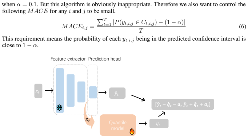
The central object is the adjustment term $a_{t,i,j}$, updated by online gradient descent on the pinball (quantile) loss, using a lagged coverage indicator because the outcome at step $j$ is only observed $j$ time steps later. The predicted quantile $\hat{q}_{t,i,j}$ from a feature-fitted quantile model serves as a time-varying offset, so the online algorithm only needs to track the residual between $\hat{q}$ and the true quantile. The key identity used in the proof is the quantile-loss gradient identity: the derivative of the pinball loss with respect to $a$ is $(1-\alpha) - I(y \in \text{interval})$, which links the update rule directly to the coverage indicator.
What would settle it
On a dataset with many repeated or discrete residual values, compute the local coverage of FFDCI over time and compare with the target 90%. If the residual distribution has a point mass at the quantile, the MACE may not shrink as predicted by Theorem 3.4. Additionally, checking whether the actual coverage gap exceeds the bound from Theorem 3.2 for small $T$ on a simple synthetic autoregressive process would test the coverage theorem directly.
Extended reading notes
Core claim
The paper claims that the problem of maintaining valid online prediction intervals can be separated into two easier pieces: predicting the quantile of the absolute error from the deep model's features, and learning only the residual between that predicted quantile and the true quantile through a simple online update. Its Theorem 3.2 shows that for every dimension and horizon, the average coverage over time converges to $1-\alpha$ at a rate of $O((M+\gamma)/(T\gamma) + (j+1)/T)$, relying on bounded errors. Its Theorem 3.4 further claims that the mean absolute coverage error over time is bounded by a constant times the square root of the RMSE of the true minus predicted quantiles plus a horizon-dependent term. The upshot is that the interval length is determined by deep features where they are informative, while the online adjustment guarantees validity without model retraining.
Load-bearing premise
The MACE bound assumes the residual distribution has a density that is bounded below by a positive constant near the quantile, so if the residual has atoms or near-zero density at that point, the claimed quadratic lower bound fails and the MACE guarantee does not follow.
Editorial extensions
If this is right
- If the coverage theorem holds, any pretrained deep forecasting model can be wrapped with FFDCI to produce valid intervals without retraining, with the same coverage guarantee for every dimension and every horizon.
- The MACE bound implies that better feature-based quantile models lead to tighter intervals while maintaining coverage, so improvements in representation quality directly translate into less uncertainty waste.
- Because the update only needs the lagged coverage indicator, the method applies to multi-step forecasting with a fixed horizon and does not require a streaming error signal at every step.
- The framework's coverage guarantee holds under distribution shift, provided the error process remains bounded, making it applicable to non-stationary forecasting settings.
- The ablation suggests that the two components play complementary roles: the online adjustment maintains coverage when the quantile model is misspecified or the distribution shifts, while the feature-fitted quantile model shortens intervals.
Reading between the lines
- A natural extension would be to use more flexible quantile models (e.g., recurrent networks) or to replace the quantile loss with a smoothed surrogate, possibly yielding tighter interval lengths while retaining the same type of coverage bound.
- The theorem's dependence on RMSE of the quantile residual suggests that one could actively select features or quantile models by minimizing this RMSE on a validation set, which may provide a principled way to choose among candidate quantile predictors.
- The bound also suggests that a quantile model that is periodically updated online could further reduce MACE, although this would require additional analysis beyond the current fixed-model assumption.
- The method's lack of explicit handling of regime shifts suggests that incorporating change-point detection or adaptive resetting of the adjustment term could improve robustness in highly non-stationary environments.
Signed reviews
Editorial analysis
A structured set of objections, weighed in public.
Referee Report
Summary. FFDCI is a conformal wrapper for frozen deep multivariate multi-horizon point forecasters. A quantile model is fit once on validation-set residuals, using features extracted by the point forecaster as inputs; during deployment the interval for each dimension and horizon is ŷ ± (q̂ + a), where a is an adjustment term updated online from realized coverage. The paper claims Theorem 3.2, per-dimension and per-horizon empirical coverage converging to 1−α at rate O((M+γ)/(Tγ) + j/T), and Theorem 3.4, Mean Absolute Coverage Error bounded by O(√(σ(q*−q̂) + M(j+1)/T)), where σ(q*−q̂) is the RMSE of the feature-based quantile fit. Experiments on 12 datasets with three base forecasters (iTransformer, Leddam, SOFTS) compare coverage, interval length, worst-dimension, and worst-horizon coverage against ECI, TQA-E, LPCI, CF-SST, ACI, PID, SPCI, FCP, and others, with ablations and sensitivity analyses.
Significance. The paper addresses a real need: converting a pretrained deep time series forecaster into one that emits per-dimension, per-horizon confidence intervals without retraining. The design is sensible, combining the ACI update with offline feature-based quantile regression; if the theorems were correct, the MACE bound would provide a clean statement that interval efficiency inherits the quality of the quantile fit. The empirical effort is substantial and a strength of the paper: 12 datasets × 3 base models with ablations, learning-rate and hidden-size sensitivity studies, MC-dropout and quantile-regression comparisons, and a released code repository. The weakness is the theoretical core, which as submitted is internally inconsistent: the coverage theorem is not proved for the algorithm printed in the paper, and the MACE proof rests on an unstated density assumption and contains inequality-direction errors. The central idea is defensible, but the current version does not support its stated claims.
major comments (4)
- [§2.4, Algorithm 1, Eq. (11), §D.1] The update rule is inconsistent across Algorithm 1, Eq. (11), Lemma D.1, and the proof of Theorem 3.2, and the printed pseudocode is the wrong one. Algorithm 1 sets a_{t+1,i,j} = a_{t,i,j} + γ(I(y_{t,i,j}∈C_{t,i,j}) − α), which grows the interval after a cover and shrinks it after a miss, while Eq. (11) and the prose specify a_{t+1,i,j} = a_{t,i,j} + γ(1 − I(y_{t,i,j}∈C_{t,i,j}) − α), the opposite direction. In addition, §2.4 correctly states that I(y_{t,i,j}∈C_{t,i,j}) is unobservable until t+j, and Lemma D.1 works with the delayed indicator I(y_{t−j,i,j}∈C_{t−j,i,j}), but Algorithm 1 uses the undelayed indicator. The telescoping identity in the proof of Theorem 3.2, I(y_{t,i,j}∈C_{t,i,j}) = (a_{t+j+1,i,j} − a_{t+j,i,j})/γ + (1−α), has yet another sign relative to Eq. (11) and corresponds to an update of the form a_{t+1} = a_t + γ(I_{t−j} − (1−α)). Under Algorithm 1's sign, the boundedness argument in Lemma D.1 fails: a term that keeps growing after every covered step and shrinking after every miss is not bounded, so the coverage guarantee cannot hold for the pseudocode as printed. The theorem as proved applies to a delay-corrected update with the sign of Eq. (11), not to Algorithm 1; the central claim is therefore unsupported for the described method, although the intended rule is identifiable and presumably fixable.
- [Theorem 3.4, Assumption 3.3, §D.2 (Eqs. 47–53)] The proof of Theorem 3.4 relies on a condition that is not stated in Assumption 3.3. In Step 2 (Appendix D, Eq. (52)), the inequality ∫_a^{a*} (β−a)p(β)dβ ≥ (p1/2)(a−a*)² requires a positive lower bound p1 on the conditional density p(β) over the whole interval between a and a*; for residual distributions with atoms or near-zero density at the quantile, this fails and the bound in Eq. (53) does not follow. Step 2 is also internally inconsistent: Eq. (47) claims an upper bound E[l(β,a) − l(β,a*)] ≤ (p2/2)(a−a*)², while Eq. (52) derives a lower bound ≥ (p1/2)(a−a*)², and Eq. (53) then substitutes the lower bound while using the wrong constant (p1/2 where the direction requires 2/p1). The proof further inserts this conditional-expectation inequality into the sum of realized losses in Eq. (46) without taking an expectation, so Theorem 3.4 as stated is not established.
- [Theorem 3.2 proof, §D.1, Eqs. (24)–(28), Lemma D.1] There are additional algebra and indexing errors in the coverage proof. Substituting Eq. (26) into Eq. (25) gives |(a_T − a_{j+1})/(Tγ) − (1−α)(j+1)/T| + (j+1)/T, which is bounded by 2(M+γ)/(Tγ) + (2−α)(j+1)/T; the move from Eq. (27) to Eq. (28) discards the (1−α)(j+1)/T term without justification, so the stated constant is too small on the j/T term (the asymptotic O((M+γ)/(Tγ) + j/T) claim itself survives). In Lemma D.1, Case 2 bounds a_{t+1} by a_t + γ(1−α) ≤ M + γ(1−α), implicitly using a_t ≤ M whereas the induction hypothesis only gives a_t ≤ M + γ, and Case 1 concludes a lower bound for a_{t+1} by comparing with a_{t−j} without justifying a_t ≥ a_{t−j}; the lemma is likely true for the delayed update, but the proof as printed is not.
- [§4.2, Tables 1 and 10] The definition of experimental validity is ad hoc and affects the headline empirical claim. Table 1 declares methods 'valid' when overall coverage exceeds 88%, although the nominal target is 90%; FFDCI itself falls to 87.3% on ETTh2 and 88.6% on traffic, while several baseline entries at 88.4% are counted as valid, and the paper reports neither standard errors nor the per-dataset spread of coverage around the 88% line. In addition, Table 10 contains implausible entries (ETTm2/leddam ACI = 0.011 and electricity/leddam ACI = 0.756, against neighboring values near 0.10 and 0.07), which weakens the claim that FFDCI has the smallest approximate MACE in most cases.
minor comments (6)
- [§2.2–§2.3, Algorithm 1] Notation for the dimensions is inconsistent: the prediction horizon is s in §2.2 but d1 elsewhere, the feature dimension is d2 in §2.2 but d1 in §2.3 and Algorithm 1, and Eq. (4) divides by T×s×p while intervals are p×d1 matrices; please harmonize these symbols.
- [Eqs. (1), (14)] The definition of σ(q*_{i,j} − q̂_{i,j}) in Eq. (14) averages over t but carries only the (i,j) subscript, and the summand in Eq. (1) uses P(y_t∈C_t) without indicating the dependence on t; the notation should be made explicit.
- [§3.2, last paragraph] The claimed advantage over a constant quantile (q̂ constant) is not formalized: the text asserts that the MACE bound would then involve σ(q*) and that a better-fit q̂ gives an improvement, but no theorem states or proves this comparison under the same assumptions.
- [§4.2, Appendix H] The MACE in Eq. (6) is defined through the true conditional coverage probability P(y_t∈C_t), which the paper acknowledges is unobservable; however, no argument connects the 100-step local-coverage proxy of Appendix H to this probability, so the experimental support for Theorem 3.4 is indirect.
- [Theorem 3.4] Theorem 3.4 bounds deployment-time MACE by σ(q* − q̂), where q* is the unobservable true conditional quantile; the paper's suggestion that σ 'could be regarded as the RMSE of quantile regression' refers to a validation-fit quantity, which need not equal the deployment-time σ under distribution shift, so the practical content of the bound is limited.
- [Throughout] There are numerous typos and naming inconsistencies: 'DDFCI' vs 'FFDCI' in Table 1 and Appendix I, 'week assumptions' (§3), 'donated as' (§2.1), 'holp' (Conclusion), 'last raw' (Appendix I), 'competitve' (Appendix F.1), and the garbled display of Eq. (12).
Circularity Check
No circularity found: the coverage and MACE guarantees are derived from the ACI-style update and quantile-fit RMSE, not from the target quantities themselves.
full rationale
I walked the paper's derivation chain. Theorem 3.2 is proved by telescoping the bounded adjustment sequence defined in Eq. (11), with the lag j entering through the delayed coverage indicators; this does not define coverage in terms of itself. Theorem 3.4 bounds MACE by combining a Lipschitz assumption on P(cover) as a function of a_t with a regret bound on the pinball loss, ending with the RMSE sigma(q* - qhat) of the feature-fitted quantile model as an input term; the bound is conditional on that goodness-of-fit, not a restatement of it. The quantile model is fit to validation errors by pinball loss, and the deployed intervals are evaluated by fresh coverage indicators, so the fitted input and the reported metric are not the same object. No uniqueness theorem or load-bearing premise is imported from the authors' prior work; the only self-citation (Gruver et al. 2024, which includes an author of this paper) appears in the introduction as motivation about LLM retraining cost and is not load-bearing. I did note two internal correctness defects that are outside the circularity definition: Algorithm 1 prints a_{t+1}=a_t+gamma(I-alpha), whereas Eq. (11) and the proof of Theorem 3.2 use a_{t+1}=a_t+gamma(1-I-alpha); and Appendix D, Step 2 uses a lower bound p1 on the conditional density of beta that is not stated in Assumption 3.3. These affect whether the stated theorem matches the implemented algorithm, but neither reduces a prediction to its input by construction. Consequently, no significant circularity is present.
Assumptions & free parameters
free parameters (2)
- gamma =
0.002 in main experiments; tuned to 0.01 for ETTh2
- quantile model hyperparameters =
MLP hidden sizes 512 and 256, learning rate 0.001, 100 epochs
assumptions (4)
- domain assumption Errors and predicted quantiles are bounded by M (Assumption 3.1)
- domain assumption Coverage probability P(y in C) is L-Lipschitz in the offset a (Assumption 3.3)
- ad hoc to paper Conditional density p(beta) has a positive lower bound p1 in the relevant interval
- standard math Convexity and regret bounds for online subgradient descent on pinball loss
Cite this review
Pith. "Pith review of Feature Fitted Online Conformal Prediction for Deep Time Series Forecasting Model." pith.science (2026). https://pith.science/paper/RL5NJHPJ
@misc{pith2026250508158,
  author       = {Pith},
  title        = {Pith review of: Feature Fitted Online Conformal Prediction for Deep Time Series Forecasting Model},
  year         = {2026},
  howpublished = {\url{https://pith.science/paper/RL5NJHPJ}},
  note         = {Machine review of arXiv:2505.08158}
}
read the original abstract
Time series forecasting is critical for many applications, where deep learning-based point prediction models have demonstrated strong performance. However, in practical scenarios, there is also a need to quantify predictive uncertainty through online confidence intervals. Existing confidence interval modeling approaches building upon these deep point prediction models suffer from key limitations: they either require costly retraining, fail to fully leverage the representational strengths of deep models, or lack theoretical guarantees. To address these gaps, we propose a lightweight conformal prediction method that provides valid coverage and shorter interval lengths without retraining. Our approach leverages features extracted from pre-trained point prediction models to fit a residual predictor and construct confidence intervals, further enhanced by an adaptive coverage control mechanism. Theoretically, we prove that our method achieves asymptotic coverage convergence, with error bounds dependent on the feature quality of the underlying point prediction model. Experiments on 12 datasets demonstrate that our method delivers tighter confidence intervals while maintaining desired coverage rates. Code, model and dataset in \href{https://github.com/xiannanhuang/FFDCI}{Github}
Figures


Figures from the paper (11 more)




Reference graph
Works this paper leans on
-
[2]
contains an indicator function that determines whether st exceedsqt. The authors argue that this indicator function is excessively non-smooth and propose replacing it with a sigmoid function. Consequently, they derive the following updated formulation forqt: qt+1 =qt +γ(errt−α− (st−qt)∇f(st−qt)) (15) whereerrt = I(st >q t),f means sigmoid function,i.e.,f(...
work page 2022
-
[3]
Softs: Efficient multivariate time series forecasting with series-core fusion
Han, L., Chen, X.-Y ., Ye, H.-J., and Zhan, D.-C. Softs: Efficient multivariate time series forecasting with series-core fusion. In NeurIPS 2024,
work page 2024
-
[7]
Bellman conformal inference: Calibrating prediction intervals for time series
11 Yang, Z., Candès, E., and Lei, L. Bellman conformal inference: Calibrating prediction intervals for time series. arXiv preprint arXiv:2402.05203,
-
[8]
Ye, J., Zhang, W., Yi, K., Yu, Y ., Li, Z., Li, J., and Tsung, F. A survey of time series founda- tion models: Generalizing time series representation with large language mode. arXiv preprint arXiv:2405.02358,
-
[9]
The Benefit of Being Bayesian in Online Conformal Prediction
Zhang, Z., Bombara, D., and Yang, H. Discounted adaptive online learning: Towards better regular- ization. In Forty-first International Conference on Machine Learning, 2024a. Zhang, Z., Lu, Z., and Yang, H. The benefit of being bayesian in online conformal prediction. arXiv preprint arXiv:2410.02561, 2024b. Zhao, R., Tian, Z., Tian, L., Liu, W., and Wang,...
-
[10]
12 A Related Work A.1 Conformal prediction and its single variable time series version The simplest version of conformal prediction is just regarding errors in validation set as the errors in test set Shafer & V ovk (2008). Therefore, if the 90 percentage quintile of errors in the validation set isq, and ˆy is a point prediction in the test set, then the ...
work page 2008
-
[14]
Besides, we used Adam to train these models for 50 epochs with early stop if loss in validation set did not decrease for 5 epochs. The learning rate was 0.001. Other hyperparameters were set as default values according to their github repositions. C Baseline methods In this section, we first introduce each baseline method and finally provide some discussi...
work page 2025
-
[17]
We also color the best performance red. It can be concluded from this table that the performance of our method is generally stable with different hidden sizes. And in many cases, increasing the hidden size to 1024 might slightly improve the results. G Results of other methods We also conducted experiments about Monte-Carlo Dropout Gal & Ghahramani (2015) ...
work page 2015
Show all 19 references
-
[18]
This pattern is consistent with experiments in Lin et al
26 Table 7: Results of sensitive analysis experiments of hidden size Hidden size 256 512 1024 Dataset Base model Cov l M in _d M in_t Cov l M in _d M in_t Cov l M in _d M in_t iTransformer 89.3% 1.681 86.6% 87.9% 89.9% 1.758 87.5% 88.3% 89.8% 1.703 87.4% 88.4% Leddam 89.3% 1.6...
2022
-
[19]
We can observe that directly using quantile regression makes it difficult to guarantee coverage
And the coverage below 50% is colored in purple. We can observe that directly using quantile regression makes it difficult to guarantee coverage. For example, the coverage for the weather dataset does not even reach 80%. Furthermore, when examining the coverage for the worst d...
2024
-
[23]
18 D.2 Proof of Theorem 3.4 Proof. Similar to to Gibbs & Candès (2024), we first defineβt,i,j as: βt,i,j =min :{β :yt,i,j∈ [ˆyt,i,j−βt,i,j− ˆqt,i,j, ˆyt,i,j +βt,i,j + ˆqt,i,j]} and we definea∗ t,i,j + ˆqt,i,j as the true 1−α quantile ofyt,i,j− ˆyt,i,j, therefore, P (yt,i,j∈ [ˆ...
2024
-
[2016]
• Solar: Solar power production data from 137 photovoltaic plants in 2006 was collected every 10 minutes
• Electricity: Hourly electricity consumption data from 321 clients was recorded. • Solar: Solar power production data from 137 photovoltaic plants in 2006 was collected every 10 minutes. • ETT: Data on 7 factors of electricity transformers was collected from July 2016 to July
2006
-
[2017]
Kernel-based optimally weighted conformal prediction intervals.arXiv preprint arXiv:2405.16828,
Lee, J., Xu, C., and Xie, Y . Kernel-based optimally weighted conformal prediction intervals.arXiv preprint arXiv:2405.16828,
-
[2018]
• PEMS: Public traffic network data from California was sampled in 5-minute windows
Four subsets are available: ETTh1 and ETTh2, recorded every hour, and ETTm1 and ETTm2, recorded every 15 minutes. • PEMS: Public traffic network data from California was sampled in 5-minute windows. For more information about datasets, please refer to Liu et al. (2024). B.2 Ba...
2024
-
[2020]
• Traffic: Hourly road occupancy rates were recorded from 862 sensors installed on freeways in the San Francisco Bay Area, covering the period from January 2015 to December
2015
-
[2021]
and Yu, R
Sun, S. and Yu, R. Copula conformal prediction for multi-step time series forecasting. arXiv preprint arXiv:2212.03281,
-
[2022]
ISBN 9781713871088
Curran Associates Inc. ISBN 9781713871088. Batra, D., Mercuri, S., and Khraishi, R. Conformal predictions for longitudinal data. arXiv preprint arXiv:2310.02863,
-
[2023]
Timesnet: Temporal 2d-variation modeling for general time series analysis
Wu, H., Hu, T., Liu, Y ., Zhou, H., Wang, J., and Long, M. Timesnet: Temporal 2d-variation modeling for general time series analysis. arXiv preprint arXiv:2210.02186,
-
[2024]
Weather4cast at neurips 2022: Super-resolution rain movie prediction under spatio-temporal shifts
Gruca, A., Serva, F., Lliso, L., Rípodas, P., Calbet, X., Herruzo, P., Pihrt, J., Raevskyi, R., Šimánek, P., Choma, M., et al. Weather4cast at neurips 2022: Super-resolution rain movie prediction under spatio-temporal shifts. In NeurIPS 2022 Competition Track, pp. 292–313. PMLR,
2022
Reviewed August 15, 2026 · model on record in the stance chip above.
Discussion (0). Continue with ORCID to comment.