REVIEW 4 major objections 6 minor 33 references
Emergence of Structure in Ensembles of Random Neural Networks
T0 review · 4 major / 6 minor · reviewed 2026-08-15 · deepseek-v4-flash
Pith's one-line read A Gibbs-weighted ensemble of random perceptrons has a finite optimal inverse temperature, $\beta^* = \pi\sqrt{d-2}$, which the paper proves is independent of the teacher vector, the number of classifiers, and the dataset size.
desk verdict A clean, novel empirical finding with an overclaimed proof: the optimal Gibbs temperature for random ensembles is real, but the CLT in Appendix A does not establish beta* = pi*sqrt(d-2). read the letter →
The pith
A machine-rendered reading of the paper's core claim, the machinery that carries it, and where it could break.
The reading
What carries the argument
The load-bearing object is the Gibbs measure over the random classifiers: each perceptron with weight vector $w_i$ receives a vote weight $\alpha_i(\beta) \propto \exp(-\beta L(\phi(w_i)))$, so the loss acts as an energy and $\beta$ as an inverse temperature. The argument then replaces the empirical average over the $n$ sampled classifiers by a Gaussian random variable via the Central Limit Theorem, applied to $Y_i = \exp\bigl(\tilde{\beta}\,\mathbb{E}_{x'}[\operatorname{sign}(w_*^T x'\, x'^T w_i)]\bigr)\, \operatorname{sign}(w_*^T x\, x^T w_i)$, where $\tilde{\beta} = \beta/2$. The mean and variance of $Y$ are evaluated using Grothendieck's identity, $\mathbb{E}_{x'}[\operatorname{sign}(w_*^T x'\, x'^T w)] = \tfrac{2}{\pi}\arcsin\bigl(w_*^T w / \lVert w\rVert\bigr)$, together with a concentration result that the inverse norm $1/\lVert w\rVert$ concentrates around $1/\sqrt{d-2}$, allowing the arcsin to be linearized. These steps produce the function $\xi(\beta)$ whose maximizer is $\beta^* = \pi\sqrt{d-2}$.
What would settle it
Fix $d$ and sample many independent weight matrices $W$ and test points $x$. For a given teacher $w_*$, compute the empirical ensemble 0-1 loss at $\beta = \pi\sqrt{d-2}$ and at, say, $0.5\,\pi\sqrt{d-2}$. If, averaged over realizations, the loss at the predicted $\beta$ is not below the loss at neighboring values, or if the location of the empirical minimum shifts systematically with $n$ or with the choice of $w_*$, the universality claim fails. A sharper test is to repeat the measurement with two structurally different teachers and check whether the empirical minimizer coincides.
Extended reading notes
Core claim
On the paper's own terms, the discovery is that the Gibbs-weighted random perceptron ensemble has a single optimal inverse temperature, $\beta^* = \pi\sqrt{d-2}$, and that this value is universal: it depends only on the ambient dimension $d$ of the input space. The ensemble classifier is $\operatorname{sign}\bigl(\sum_i \exp(-\beta L(\phi(w_i)))\, \phi(w_i)(x)\bigr)$, with $w_i \sim \mathcal{N}(0, I_d)$, $L$ the 0-1 loss, and $\phi(w)(x) = \operatorname{sign}(w^T x)$. For data $x \sim \mathcal{N}(0, I_d)$ with labels $y = \operatorname{sign}(w_*^T x)$, the paper derives the loss profile through a Central Limit Theorem approximation, identifies its minimizer in closed form, and confirms numerically that the minimum is unchanged when the teacher $w_*$, the number of classifiers $n$, or the number of samples $N$ are varied. The same qualitative finite-temperature minimum is observed on MNIST for three different label tasks at essentially the same $\beta^*$, suggesting the phenomenon extends beyond isotropic Gaussians.
Load-bearing premise
The proof's central approximation is that the average over classifiers of $Y_i$ is Gaussian with the independent-sample variance $(1/n)\operatorname{Var}(Y)$, although every $Y_i$ shares the same test point $x$; if the correlations induced by $x$ are not negligible at the studied $d$ and $n$, the predicted $\beta^*$ need not minimize the actual loss.
Editorial extensions
If this is right
- At $\beta^* = \pi\sqrt{d-2}$, an untrained random perceptron ensemble classifies Gaussian teacher data near its best attainable performance, so no validation-set tuning of the temperature is needed on such data.
- The value $\beta^*$ is invariant under changes of teacher, ensemble size $n$, and sample size $N$, so the optimal weighting is a function of the data geometry alone in the isotropic Gaussian case.
- The same finite-temperature optimum appears on MNIST for three distinct binary tasks, indicating that the mechanism is not an artifact of Gaussian symmetry and may apply to structured real-world data.
- Because $\beta^*$ grows as $\sqrt{d}$, higher-dimensional inputs call for sharper weighting of low-loss classifiers even when $n$ and $N$ are held fixed.
- The perceptron-merging approximation collapses the ensemble to a single weight vector $w_{\mathrm{ens}} = \sum_i \alpha_i w_i$ with nearly unchanged accuracy, reducing inference cost to one dot product.
Reading between the lines
- Editorial inference: if the universality of $\beta^*$ survives moderately non-Gaussian data, the temperature could serve as a default hyperparameter in random-feature and reservoir models, replacing cross-validated temperature searches.
- Editorial inference: the i.i.d. Central Limit Theorem step suggests the approximation is safest when $n$ is large relative to the correlation length induced by $x$; an explicit finite-$n$ correction or a conditional CLT would show whether $\beta^* = \pi\sqrt{d-2}$ is only the leading term of a series in $1/\sqrt{n}$.
- Editorial inference: on low-intrinsic-dimension data like MNIST, the relevant $d$ in $\beta^* = \pi\sqrt{d-2}$ may be the intrinsic dimension rather than the ambient dimension; studying synthetic data with known intrinsic dimension would test whether the formula transfers.
Signed reviews
Editorial analysis
A structured set of objections, weighed in public.
Referee Report
Summary. The paper studies a Gibbs-weighted ensemble of random perceptrons, with classifier weights proportional to exp(-β times the 0-1 loss), and claims that for Gaussian teacher-perceptron data the optimal inverse temperature is β* = π√(d-2), independent of the teacher vector, the number of classifiers n, and the dataset size N. The claim is supported by loss-profile experiments in Section 3, a heuristic analytic derivation in Appendix A, and MNIST experiments in Section 4, and a minimal working example is provided.
Significance. The empirical observation of a finite optimal temperature is clean and clearly documented, and the apparent independence of the optimum from the teacher and from n and N is striking. The manuscript ships a minimal working example and the core numerical results appear reproducible. However, the analytic proof in Appendix A relies on an unjustified central-limit step and on uncontrolled asymptotic approximations; as it stands, the closed form β* = π√(d-2) is a numerically supported conjecture rather than a theorem.
major comments (4)
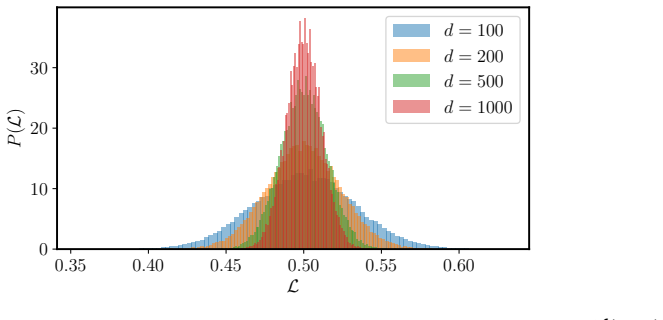
- [Appendix A, CLT step] The line "We can therefore study the sum as a normally distributed random variable, thanks to the Central Limit Theorem" is not justified, because the variables Y_i share the same test point x and are only conditionally i.i.d. given x. Writing m(x) = E_w[Y|x] and v(x) = Var_w(Y|x), the exact variance of n^{-1}Σ_i Y_i is Var_x[m(x)] + n^{-1}E_x[v(x)], whereas the unconditional CLT used in the paper gives n^{-1}Var_{x,w}Y = n^{-1}(Var_x[m(x)] + E_x[v(x)]). The term Var_x[m(x)] does not decay with n, and in the regime of Figure 4 (d=500, n=20000) it is of order 1/d while the sampling term is of order 1/n; the omitted term is numerically dominant. Consequently the derivation of ξ(β) and of β* = π√(d-2) in Eqs. (2)-(3) does not go through as written.
- [Abstract and Section 3] Because of the issue in Appendix A, the statement in the Abstract and Section 3 that the optimal temperature is "analytically prove[n]" is not supported. The closed form β* = π√(d-2) should be presented as a numerically verified conjecture unless a correct derivation is supplied; the current proof is load-bearing for the paper's central theoretical contribution.
- [Appendix C] The approximations arcsin(A) ≈ A and 1/||w|| ≈ E[1/||w||] are used without error bounds. The claim following Eq. (4) is supported only by numerical evidence, and these approximations enter the exponential arguments defining μ and σ² in Appendix A. Since the maximizer of ξ(β) depends on those arguments, the closed form β* is not rigorously controlled by the presented analysis.
- [Section 3, Figure 4b] The empirical claim that β* is independent of n is checked at only three values (n=100, 5000, 20000) for a single d. Under the correct variance decomposition of the ensemble average, the relative contribution of Var_x[m(x)] versus n^{-1}E_x[v(x)] changes with n, so these three points are too sparse to establish n-independence, especially because the present theory incorrectly predicts n-independence through cancellation of the √n factor in ξ(β).
minor comments (6)
- [Abstract and Section 3] There are several typos and grammatical issues: "does not depend neither" should be "does not depend on either," "wether" should be "whether," and the Figure 3 caption contains "minimmum" for "minimum."
- [Section 1, Eq. (1)] The notation for the weights is inconsistent: α_w(β) is defined for a single classifier, but later α_W(β) is used as a vector, and the normalization by the partition function Z_n(β) is not made explicit in Eq. (1). Please clarify the notation.
- [Appendix A] The phrase "an affine transformation x ↦ 2(-x + 1/2)" is not a well-defined affine map on R^d as written, and the claim that affine transformations cannot alter the number or position of critical points is confusing; the change of variables should be rewritten carefully.
- [Appendix C] The identity used for E_{x} sign(w_*^T x x^T w) is attributed to "Grothendieck's Identity" via reference [32]; a more specific citation or statement of the identity would help the reader verify the step.
- [Figure 4] The axis labels in Figure 4 are minimal, and it is not immediately clear which curve corresponds to which fixed parameter in each panel; please add legend entries or annotate the panels with the fixed values of the other parameters.
- [Appendix E] The Python code in Code Snippet 1 contains inconsistent spacing in variable names such as "t r a i n _ s e e d" and "te st _s ee d"; this is likely a formatting artifact but should be cleaned up for reproducibility.
Circularity Check
No circularity: the optimal-temperature formula is derived from a self-contained model and checked against simulations, not fitted.
full rationale
The paper's central claim, β* = π√(d−2), is obtained from a self-contained analytical model in Appendix A. The ensemble vote is expressed as the sign of an average of identically distributed random variables, and the mean and variance of that average are computed using standard external facts: Grothendieck's identity, the moment generating function of a Gaussian, and inverse-chi-square concentration of the norm. No parameter is fitted to the numerically observed loss minima; the function ξ(β) is derived from the model, and its maximizer is computed by differentiation in Appendix B, then compared with independently simulated minima in Figure 6. The paper contains no self-citations, invokes no uniqueness theorem from the authors' prior work, and adopts no ansatz from a self-citation chain. The only identifiable weakness is the unconditional CLT step in Appendix A, which treats the classifier-dependent variables as i.i.d. while ignoring the shared test point x; that is a technical approximation and a correctness risk, not a circular reduction of the prediction to its own inputs. Since the predicted β* is not constructed from the empirical quantities it is meant to explain, the derivation is not circular.
Assumptions & free parameters
assumptions (4)
- domain assumption Data are drawn from an isotropic Gaussian distribution x ~ N(0, I_d) and labels are generated by a teacher perceptron sign(w_*^T x) with ||w_*|| = 1.
- domain assumption The ensemble operates in the infinite-data regime: the per-classifier loss L_i is the population expectation E_{x'}[1_{...}] rather than a finite-sample mean.
- ad hoc to paper The sample average of the Y_i variables is normally distributed with mean E_{x,w}[Y] and variance (1/n) Var_{x,w}[Y], i.e., the Y_i are treated as i.i.d. even though the test point x is shared across classifiers.
- domain assumption High-dimensional concentration permits replacing 1/||w|| by 1/sqrt(d-2) and linearizing arcsin(A) approximately A.
Cite this review
Pith. "Pith review of Emergence of Structure in Ensembles of Random Neural Networks." pith.science (2026). https://pith.science/paper/46KJ3P5C
@misc{pith2026250510331,
  author       = {Pith},
  title        = {Pith review of: Emergence of Structure in Ensembles of Random Neural Networks},
  year         = {2026},
  howpublished = {\url{https://pith.science/paper/46KJ3P5C}},
  note         = {Machine review of arXiv:2505.10331}
}
read the original abstract
Randomness is ubiquitous in many applications across data science and machine learning. Remarkably, systems composed of random components often display emergent global behaviors that appear deterministic, manifesting a transition from microscopic disorder to macroscopic organization. In this work, we introduce a theoretical model for studying the emergence of collective behaviors in ensembles of random classifiers. We argue that, if the ensemble is weighted through the Gibbs measure defined by adopting the classification loss as an energy, then there exists a finite temperature parameter for the distribution such that the classification is optimal, with respect to the loss (or the energy). Interestingly, for the case in which samples are generated by a Gaussian distribution and labels are constructed by employing a teacher perceptron, we analytically prove and numerically confirm that such optimal temperature does not depend neither on the teacher classifier (which is, by construction of the learning problem, unknown), nor on the number of random classifiers, highlighting the universal nature of the observed behavior. Experiments on the MNIST dataset underline the relevance of this phenomenon in high-quality, noiseless, datasets. Finally, a physical analogy allows us to shed light on the self-organizing nature of the studied phenomenon.
Figures


Figures from the paper (7 more)


Reference graph
Works this paper leans on
-
[1]
A review on neural networks with random weights,
W. Cao, X. Wang, Z. Ming, and J. Gao, “A review on neural networks with random weights,” Neurocomputing, vol. 275, pp. 278–287, 2018
work page 2018
-
[2]
C. M. Bishop and N. M. Nasrabadi, Pattern recognition and machine learning, vol. 4. Springer, 2006
2006
-
[3]
R. Couillet and Z. Liao, Random matrix methods for machine learning. Cambridge University Press, 2022
work page 2022
-
[4]
Backpropagation and stochastic gradient descent method,
S.-i. Amari, “Backpropagation and stochastic gradient descent method,”Neurocomputing, vol. 5, no. 4-5, pp. 185–196, 1993
1993
-
[5]
Engel, Statistical mechanics of learning
A. Engel, Statistical mechanics of learning. Cambridge University Press, 2001
work page 2001
-
[6]
On weight initialization in deep neural networks,
S. K. Kumar, “On weight initialization in deep neural networks,” arXiv preprint arXiv:1704.08863, 2017
arXiv 2017
-
[7]
A review on weight initialization strategies for neural networks,
M. V . Narkhede, P. P. Bartakke, and M. S. Sutaone, “A review on weight initialization strategies for neural networks,” Artificial intelligence review, vol. 55, no. 1, pp. 291–322, 2022
work page 2022
-
[8]
Eigenvalues of covariance matrices: Application to neural-network learning,
Y . Le Cun, I. Kanter, and S. A. Solla, “Eigenvalues of covariance matrices: Application to neural-network learning,” Physical review letters, vol. 66, no. 18, p. 2396, 1991
work page 1991
Show all 33 references
-
[9]
Attention is all you need,
A. Vaswani, N. Shazeer, N. Parmar, J. Uszkoreit, L. Jones, A. N. Gomez, Ł. Kaiser, and I. Polosukhin, “Attention is all you need,”Advances in neural information processing systems, vol. 30, 2017
2017
-
[10]
Highly accurate protein structure prediction with alphafold,
J. Jumper, R. Evans, A. Pritzel, T. Green, M. Figurnov, O. Ronneberger, K. Tunyasuvunakool, R. Bates, A. Žídek, A. Potapenko, et al., “Highly accurate protein structure prediction with alphafold,” nature, vol. 596, no. 7873, pp. 583–589, 2021
2021
-
[11]
How does weight correlation affect generalisation ability of deep neural networks?,
G. Jin, X. Yi, L. Zhang, L. Zhang, S. Schewe, and X. Huang, “How does weight correlation affect generalisation ability of deep neural networks?,” Advances in Neural Information Processing Systems, vol. 33, pp. 21346–21356, 2020
2020
-
[12]
Heavy-tailed universality predicts trends in test accuracies for very large pre-trained deep neural networks,
C. H. Martin and M. W. Mahoney, “Heavy-tailed universality predicts trends in test accuracies for very large pre-trained deep neural networks,” inProceedings of the 2020 SIAM International Conference on Data Mining, pp. 505–513, SIAM, 2020
2020
-
[13]
Computational power of neural networks: A characterization in terms of kolmogorov complexity,
J. L. Balcázar, R. Gavalda, and H. T. Siegelmann, “Computational power of neural networks: A characterization in terms of kolmogorov complexity,” IEEE Transactions on Information Theory, vol. 43, no. 4, pp. 1175–1183, 2002
2002
-
[14]
Spin glass theory and its new challenge: structured disorder,
M. Mézard, “Spin glass theory and its new challenge: structured disorder,” Indian Journal of Physics, vol. 98, no. 11, pp. 3757–3768, 2024
2024
-
[15]
More is different: Broken symmetry and the nature of the hierarchical structure of science.,
P. W. Anderson, “More is different: Broken symmetry and the nature of the hierarchical structure of science.,” Science, vol. 177, no. 4047, pp. 393–396, 1972
1972
-
[16]
The perceptron: A model for brain functioning. i,
H.-D. Block, “The perceptron: A model for brain functioning. i,” Reviews of Modern Physics, vol. 34, no. 1, p. 123, 1962
1962
-
[17]
Huang, Statistical mechanics
K. Huang, Statistical mechanics. John Wiley & Sons, 2008
2008
-
[18]
Mnist handwritten digit database,
Y . LeCun, C. Cortes, and C. Burges, “Mnist handwritten digit database,”ATT Labs [Online]. Available: http://yann.lecun.com/exdb/mnist, vol. 2, 2010
2010
-
[19]
Emerging opportunities and challenges for the future of reservoir computing,
M. Yan, C. Huang, P. Bienstman, P. Tino, W. Lin, and J. Sun, “Emerging opportunities and challenges for the future of reservoir computing,” Nature Communications, vol. 15, no. 1, p. 2056, 2024
2024
-
[20]
A review on extreme learning machine,
J. Wang, S. Lu, S.-H. Wang, and Y .-D. Zhang, “A review on extreme learning machine,” Multimedia Tools and Applications, vol. 81, no. 29, pp. 41611–41660, 2022
2022
-
[21]
Visual feature extraction by a multilayered network of analog threshold ele- ments,
K. Fukushima, “Visual feature extraction by a multilayered network of analog threshold ele- ments,” IEEE Transactions on Systems Science and Cybernetics, vol. 5, no. 4, pp. 322–333, 1969
1969
-
[22]
On random weights and unsupervised feature learning.,
A. M. Saxe, P. W. Koh, Z. Chen, M. Bhand, B. Suresh, and A. Y . Ng, “On random weights and unsupervised feature learning.,” in Icml, vol. 2, p. 6, 2011. 10
2011
-
[23]
Beyond simple features: A large-scale feature search approach to unconstrained face recognition,
D. Cox and N. Pinto, “Beyond simple features: A large-scale feature search approach to unconstrained face recognition,” in 2011 IEEE International Conference on Automatic Face & Gesture Recognition (FG), pp. 8 – 15, 04 2011
2011
-
[24]
Deep neural networks with random gaussian weights: A universal classification strategy?,
R. Giryes, G. Sapiro, and A. M. Bronstein, “Deep neural networks with random gaussian weights: A universal classification strategy?,” IEEE Transactions on Signal Processing, vol. 64, no. 13, pp. 3444–3457, 2016
2016
-
[25]
Deep randomized neural networks,
C. Gallicchio and S. Scardapane, “Deep randomized neural networks,” in Recent Trends in Learning From Data: Tutorials from the INNS Big Data and Deep Learning Conference (INNSBDDL2019), pp. 43–68, Springer, 2020
2020
-
[26]
Distilling the knowledge in a neural network,
G. Hinton, O. Vinyals, and J. Dean, “Distilling the knowledge in a neural network,” arXiv preprint arXiv:1503.02531, 2015
2015 arXiv
-
[27]
On the properties of the softmax function with application in game theory and reinforcement learning,
B. Gao and L. Pavel, “On the properties of the softmax function with application in game theory and reinforcement learning,” arXiv preprint arXiv:1704.00805, 2017
2017 arXiv
-
[28]
A phase transition in diffusion models reveals the hierarchical nature of data,
A. Sclocchi, A. Favero, and M. Wyart, “A phase transition in diffusion models reveals the hierarchical nature of data,” Proceedings of the National Academy of Sciences, vol. 122, no. 1, p. e2408799121, 2025
2025
-
[29]
Why and when can deep-but not shallow-networks avoid the curse of dimensionality: a review,
T. Poggio, H. Mhaskar, L. Rosasco, B. Miranda, and Q. Liao, “Why and when can deep-but not shallow-networks avoid the curse of dimensionality: a review,” International Journal of Automation and Computing, vol. 14, no. 5, pp. 503–519, 2017
2017
-
[30]
Intrinsic dimensionality estimation of submanifolds in rd,
M. Hein and J.-Y . Audibert, “Intrinsic dimensionality estimation of submanifolds in rd,” in Proceedings of the 22nd international conference on Machine learning, pp. 289–296, 2005
2005
-
[31]
Asymptotic learning curves of kernel methods: em- pirical data versus teacher–student paradigm,
S. Spigler, M. Geiger, and M. Wyart, “Asymptotic learning curves of kernel methods: em- pirical data versus teacher–student paradigm,” Journal of Statistical Mechanics: Theory and Experiment, vol. 2020, no. 12, p. 124001, 2020
2020
-
[32]
sign nX i exp ˜βEx′ h sign(wT ∗ x′x′T wi) i sign(wT ∗ xxT wi) !# , which can be rewritten, employing the identity sign(x) = 2· 1 ≥(x)− 1 that holds for everyx̸= 0, as −¯L∝ Ex,W1
R. Vershynin, High-dimensional probability: An introduction with applications in data science, vol. 47. Cambridge university press, 2018. 11 Appendix A Analytical model for the optimal β Consider the infinite data (that means that we neglect the fluctuations of the loss over v...
2018
-
[33]
Train accuracy : %.3 f
and High Dimensional Geometry and was for us a valid tool for constructing our solution of the optimalβ problem. Appendix D Perceptron merging A similar idea to the one proposed in Appendix C can be employed for averaging the contribution of the perceptrons directly in the par...
2025
Reviewed August 15, 2026 · model on record in the stance chip above.
Discussion (0). Continue with ORCID to comment.