REVIEW 3 major objections 6 minor 1 cited by
Algorithmic Hiring and Diversity: Reducing Human-Algorithm Similarity for Better Outcomes
T0 review · 3 major / 6 minor · reviewed 2026-08-07 · deepseek-v4-flash
Pith's one-line read The paper proves that equal-selection fairness constraints in algorithmic hiring lose their power as the screening algorithm's rankings converge on the hiring manager's, and shows on 799,000 applications that balancing shortlists is not…
desk verdict The core insight—equal shortlist constraints lose their power when screeners and managers agree—is real and useful, but the paper's main empirical validation is circular and needs reworking before the results can be trusted. read the letter →
The pith
A machine-rendered reading of the paper's core claim, the machinery that carries it, and where it could break.
The reading
What carries the argument
The load-bearing object is $\theta$, the correlation between the screening algorithm's score $Q_S$ and the hiring manager's score $Q_H$ inside a trivariate Gaussian model $(Q, Q_S, Q_H)$ of true quality and both evaluations. It is the single parameter that controls both results: at high $\theta$, gender gaps in shortlist scores become gender gaps in hiring scores, diluting equal selection, and the two stages become redundant signals, diluting hire quality. The proofs differentiate bivariate normal selection probabilities and truncated expectations, using Plackett's identity for the derivative of the bivariate normal cumulative distribution function with respect to correlation, together with Tallis's truncated-normal expectation formula. The complementary algorithm turns $\theta$ into a design lever: it trains on true quality to keep the algorithm accurate while choosing shortlists with minimal gender differences in predicted $Q_H$, thereby surfacing candidates who would be overlooked by the manager yet remain competitive on the manager's own criteria.
What would settle it
Take a set of job postings that use equal-selection shortlists, collect the hiring managers' actual evaluation scores rather than only binary decisions, and compute the female hire share as a function of the correlation between those scores and the screening algorithm's scores; if the female share does not decline as this correlation rises, Proposition 1's central prediction is false. A complementary experiment could randomly assign the paper's screening rules to postings, and the claim would fail if the complementary rule does not produce a higher female hire share at equal hired quality.
Extended reading notes
Core claim
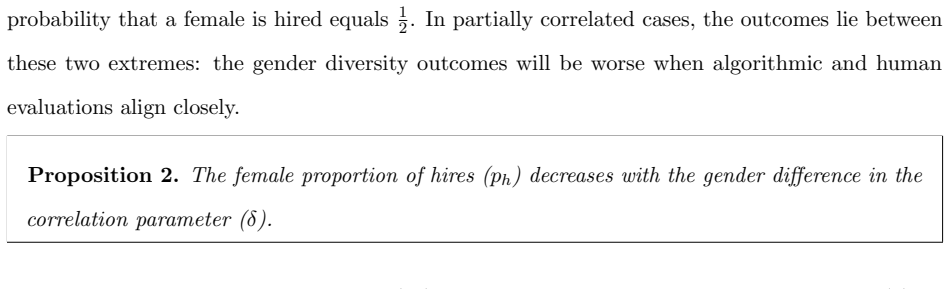
The paper's central result is Proposition 1: in a two-stage pipeline with algorithmic screening followed by a gender-unbiased human manager, the effectiveness of the equal selection constraint, measured as the female proportion of hires $p_h$, decreases as $\theta$, the correlation between the screening score $Q_S$ and the manager's score $Q_H$, increases. The corollary is sharp: at $\theta = 0$ the constraint makes hires gender-balanced, while at $\theta = 1$ it has no effect. The mechanism is that equal selection deliberately lowers the screening threshold for the underrepresented female group; if the two scores are perfectly aligned, that lower average screening score carries directly into lower managerial scores, so shortlisted women are systematically less likely to clear the final threshold. The paper also proves (Proposition 3) that conditional on how well each stage predicts true quality, expected hire quality is maximized at $\theta = 0$ and declines as $\theta$ grows, because two more-correlated signals carry more redundant information about candidate quality. Empirically, the authors estimate $\hat{\theta} \approx 0.43$ on average across 3,608 job postings and show the constraint moves female representation from 31% of applicants to 50% of shortlists but only to 41% of hires, with 36% in Engineering & Technical roles; regressions confirm the predicted negative relationship between $\theta$ and $p_h$ under the constraint.
Load-bearing premise
The empirical support rests on treating the Spearman correlation between an ML model's predicted screening probability and its predicted manager probability as the true $\theta$ between the algorithm's score and a hiring manager's actual, unobserved evaluation; if that proxy is biased, the estimated diversity gains and the test of Proposition 1 do not follow.
Editorial extensions
If this is right
- Equal selection at the shortlist is not a guarantee of equal hires: a gender-balanced shortlist yields roughly 41% female hires on average, and only 36% in engineering roles, when algorithmic and managerial scores correlate at typical levels.
- The larger the overlap between algorithm and manager criteria, the smaller the diversity gain and the lower the expected quality of hires; firms should treat the correlation $\theta$, not just predictive accuracy, as a design parameter.
- Training screening models on manager decisions or on historical screener scores that mirror them maximizes $\theta$ and therefore sacrifices the diversity benefit of fairness constraints; training on true job performance while minimizing gender gaps in predicted manager scores performs better.
- Standard group-fairness constraints, such as demographic parity, error rate parity, and equalized odds, do little to move hired-pool diversity in this data, so diversity-focused hiring pipelines need constraints aimed at the downstream human stage.
- The diversity shortfall after the shortlist is not necessarily evidence of biased managers, which matters for trust in fairness policies when post-shortlist gender gaps appear.
Reading between the lines
- Beyond the paper: the same diversity leak should appear whenever an upstream parity constraint selects on one signal and a downstream human decides on a correlated signal, for example race or age in Rooney-Rule-style policies or resume screening before interviews, so $\theta$ is a portable diagnostic across such pipelines.
- Beyond the paper: because the empirical $\theta$ is measured between two models of resume text rather than between the deployed algorithm and managers' confidential interview assessments, the true correlation may be higher than 0.43, which would make real-world equal-selection effectiveness even lower than the 41% estimate.
- Beyond the paper: a field experiment could vary how much resume-derived information a manager sees before interviewing; reducing $\theta$ this way should raise both female hire share and average hire quality, a testable prediction of the complementarity logic.
- Beyond the paper: Proposition 3's quality payoff at low $\theta$ implies a long-run quality advantage for complementary screening, because the algorithm repeatedly surfaces candidates managers would have under-ranked; diversity gains may compound rather than trade off against performance.
Editorial analysis
A structured set of objections, weighed in public.
Referee Report
Summary. The paper studies a two-stage hiring pipeline in which an algorithmic screener applies an equal-selection (gender-balanced shortlist) constraint and a human hiring manager then chooses finalists. The theoretical model assumes multivariate Gaussian latent scores (Q, QS, QH) and yields three propositions: the female share of hires under equal selection decreases with the correlation θ between algorithmic and managerial scores; it decreases with gender differences δ in that correlation; and expected hire quality decreases with θ at fixed predictive accuracies. The authors then estimate θ and δ from roughly 800,000 applications at eight technology firms using transformer-based models, simulate counterfactual policies by imputing estimated parameters into the theoretical model, and benchmark a proposed 'complementary equal selection' algorithm against standard fairness constraints. The paper's headline claims are that equal shortlists yield only modest final-hire diversity gains (ph ≈ 0.41 overall, Table 6) and that the gains decline with θ (Table 5), while the complementary algorithm substantially improves diversity with little quality loss.
Significance. If the theoretical results are rigorously established and the empirical validation were genuinely independent, the paper would make a timely and practically relevant contribution to the algorithmic fairness and human-AI hiring literatures. The scale of the dataset, the two-stage framing, and the concrete algorithmic proposal are strengths, as is the agent-based benchmarking in Section 5.4 that relaxes the Gaussian/equal-quality assumptions. The central weakness is that the main empirical test of Proposition 1 (Section 5.3, Table 5) is not independent of the theory: the outcome variable ph is itself generated by the theoretical model, so the regression recovers the model's assumed functional form rather than validating it. The theoretical proof of Proposition 1 is also informal. These issues are load-bearing for the paper's central claim, although they are potentially fixable.
major comments (3)
- [Appendix A.2, Proposition 1] The proof of Proposition 1 is not rigorous. After defining the boost function g(qS, θ) = ∂P(H|qS,θ)/∂θ, the proof asserts that because g increases in qS and the men's integration range [τ_m^S, ∞) is shifted upward relative to the women's range [τ_f^S, ∞), the relative rate N'(θ)/N(θ) is smaller than M'(θ)/M(θ). This does not follow from monotonicity of g alone; one must compare weighted averages of g against weighted averages of the hiring probability over the two truncated ranges and show the relevant ratio inequality, which the text does not do. The corollary at θ = 1 is also ambiguous: with a common hiring threshold τH, if τH lies between τ_f^S and τ_m^S, equal selection changes ph rather than having 'no effect'; the claimed behavior needs explicit conditions on τH.
- [Section 5.3, Eq. (5.1), Table 5; Table 6 note] The regression in Eq. (5.1) does not provide an empirical test of Proposition 1. As stated in the Table 6 note, ph is 'estimated by first estimating the job-specific model parameters (θ̂j, δ̂j), and imputing the model parameters into the theoretical model.' Thus the dependent variable ph,j in Table 5 is a deterministic function of θ̂j, δ̂j, pa,j, and the thresholds, and the negative θ coefficient and positive θ² coefficient reflect the imposed Gaussian truncation model rather than independent evidence. The paper should either calibrate the model's no-constraint predictions against observed finalist proportions and show the model reproduces actual outcomes, or re-run the Proposition 1 test using the non-parametric agent-based simulations from Section 5.4.
- [Section 4.3, Eq. (4.3); Section 5.4] The estimated θ is the Spearman correlation between ML-predicted screening probabilities and ML-predicted hiring-manager probabilities, but the theoretical θ is the correlation between the screening score QS and the manager's actual evaluation QH, which includes interview information not present in resumes. The manager model is trained only on binary interview outcomes of shortlisted candidates, so the proxy may be attenuated or otherwise biased. Since the same predicted qH is used both to estimate θ and as the hiring-manager agent in the Section 5.4 simulations, any bias propagates into the simulated diversity gains and the Table 5/6 conclusions. The paper should validate the proxy against observable downstream outcomes or report sensitivity analyses under alternative assumptions about the unobserved manager signal.
minor comments (6)
- [Table 5 note] The note says the model is estimated 'with (Model (2)) and without the equal selection constraint (Model (2))'; the second reference should be Model (1).
- [Appendix C.3, Table 12] The Kolmogorov-Smirnov p-values are all < 0.0001, including for the Gaussian copula, so describing the Gaussian copula as having good goodness-of-fit is overstated; the text should acknowledge that every candidate copula is rejected at conventional levels.
- [Figure 2 and Corollary 1] The figure and corollary do not state the hiring threshold τH relative to the shortlist thresholds τ_f^S and τ_m^S, but the θ=1 behavior depends on this relationship; the caption should specify the parameter values used.
- [Section 5.4, Figure 9] The statement that error bars 'are not visible because they are narrow' should be replaced with the actual bootstrapped interval widths or a note on the scale, since invisible error bars convey no information to the reader.
- [Table 4] The 'Other' category has only 214 applicants in the hold-out set yet contributes a δ estimate of -0.332; the text should flag this small-sample estimate as unreliable rather than presenting it alongside the larger categories without caveat.
- [Eq. (3.3)] The conditional entropy expression has a formatting issue: '2eπ · Det(...) / (1 − θ²)' should be written with parentheses and a factor of 2πe made explicit, and the determinant should be shown clearly.
Circularity Check
The empirical test of Proposition 1 is circular: the outcome ph in eq. 5.1 is simulated from the same Gaussian model using the fitted θ and δ, so the regression recovers the model's own assumptions rather than providing independent validation.
-
fitted input called prediction
[Section 5.2 (Table 6 note) and Section 5.3 (eq. 5.1)]
"ps and ph are estimated by first estimating the job-specific model parameters (θ̂j, δ̂j), and imputing the model parameters into the theoretical model. ... We next exploit the variation in parameter estimates across jobs to empirically test Proposition 1 and Proposition 2 using the following regression specification: ph,j = β0 + β1pa,j + β2θj + β3θj^2 + β4δj + β5δj^2 + εj"
The dependent variable ph,j in eq. (5.1) is not an observed finalist outcome; it is generated by plugging the job-specific estimates θ̂j and δ̂j into the same Gaussian-theory model whose Proposition 1 is being tested. Therefore regressing ph on θ̂ and θ̂² cannot independently confirm Proposition 1. The negative θ coefficient and the curvature are mathematical consequences of the model's construction (e.g., τf < τm with bivariate normal truncation), not evidence from the 800k applications. The data enter only through fitted parameters and thresholds; no hold-out interview or finalist outcomes constitute the outcome variable.
-
self definitional
[Section 5.4, Table 7]
"Complementary Equal Selection | P(g = f|ŷS = 1) = P(g = m|ŷS = 1); min E[q̂H_s|g = f] − E[q̂H_s|g = m] ... the hiring manager agent selects the candidates with the highest hiring manager scores, q̂H."
The complementary algorithm is defined to minimize gender differences in the predicted manager score q̂H, and the simulated manager hires according to the same q̂H scores. The reported diversity gain for Complementary Equal Selection is therefore the algorithm's own optimization objective realized in simulation: balancing q̂H between genders, followed by thresholding on q̂H, mechanically moves ph toward 0.5. This is a useful demonstration of the mechanism, but it is not an independent empirical prediction, and it inflates the evidential strength of the benchmarking result.
full rationale
The analytic derivation of Proposition 1 (Appendix A.2) is a self-contained Gaussian-truncation argument and is not itself circular. The problem is the empirical validation: Tables 5 and 6 construct the 'hired' gender proportion ph by imputing estimated θ̂j and δ̂j into the theoretical model, then regress that constructed ph on θ̂j. This makes the 'test of propositions' a deterministic check of the model's own functional form, not an independent test using actual finalist outcomes. The agent-based simulations in Section 5.4 are non-parametric and use actual candidate-level ML scores, but the paper's headline regression and aggregate Table 6 results do not rely on them, and the complementary-algorithm diversity gain in those simulations is itself partly forced by the algorithm's objective. There is no significant self-citation circularity here; the issue is that the central empirical claim reduces by construction to the model whose predictions it purports to validate. Score 6 reflects this partial but load-bearing circularity.
Assumptions & free parameters
free parameters (4)
- theta (screening-manager correlation) =
estimated per job, average 0.434
- delta (gender difference in correlation) =
estimated per job, average -0.007
- theta_S (screening accuracy) =
assumed 0.3, 0.5, 0.7
- theta_H (manager accuracy) =
assumed 0.3, 0.5, 0.7
assumptions (6)
- domain assumption Joint scores (Q, QS, QH) follow a multivariate normal distribution or a Gaussian copula after transformation.
- domain assumption No gender bias in the hiring manager stage (beta_H = 0, delta_H = 0).
- domain assumption Equal selection is implemented via gender-specific thresholds with pa < 0.5.
- ad hoc to paper ML-predicted decision probabilities, after Gaussian copula transformation, recover the latent quality scores.
- domain assumption Inverse propensity weighting removes selection bias in manager scores.
- domain assumption Hiring managers do not adapt their behavior to fairness constraints.
Cite this review
Pith. "Pith review of Algorithmic Hiring and Diversity: Reducing Human-Algorithm Similarity for Better Outcomes." pith.science (2026). https://pith.science/paper/NR32FAC6
@misc{pith2026250514388,
  author       = {Pith},
  title        = {Pith review of: Algorithmic Hiring and Diversity: Reducing Human-Algorithm Similarity for Better Outcomes},
  year         = {2026},
  howpublished = {\url{https://pith.science/paper/NR32FAC6}},
  note         = {Machine review of arXiv:2505.14388}
}
read the original abstract
Algorithmic tools are increasingly used in hiring to improve fairness and diversity, often by enforcing constraints such as gender-balanced candidate shortlists. However, we show theoretically and empirically that enforcing equal representation at the shortlist stage does not necessarily translate into more diverse final hires, even when there is no gender bias in the hiring stage. We identify a crucial factor influencing this outcome: the correlation between the algorithm's screening criteria and the human hiring manager's evaluation criteria -- higher correlation leads to lower diversity in final hires. Using a large-scale empirical analysis of nearly 800,000 job applications across multiple technology firms, we find that enforcing equal shortlists yields limited improvements in hire diversity when the algorithmic screening closely mirrors the hiring manager's preferences. We propose a complementary algorithmic approach designed explicitly to diversify shortlists by selecting candidates likely to be overlooked by managers, yet still competitive according to their evaluation criteria. Empirical simulations show that this approach significantly enhances gender diversity in final hires without substantially compromising hire quality. These findings highlight the importance of algorithmic design choices in achieving organizational diversity goals and provide actionable guidance for practitioners implementing fairness-oriented hiring algorithms.
Figures


Figures from the paper (3 more)


Forward citations
Cited by 1 Pith paper
-
A Hierarchy of Policy Learning Problems
Policy existence reduces to improving-policy learning which reduces to optimal-policy learning; under a natural monotonicity condition the first two are separated by a polynomial sample-complexity gap.
Reference graph
Works this paper leans on
-
[1]
Q, QS, QH have marginal PDFs ϕ(q), ϕ(qS), ϕ(qH )
ϕ(x) is the standard normal Probability Density Function (PDF). Q, QS, QH have marginal PDFs ϕ(q), ϕ(qS), ϕ(qH )
-
[2]
Q, QS, QH have marginal CDFs Φ( q), Φ(qS), Φ(qH )
Φ(x) is the standard normal Cumulative Distribution Function (CDF). Q, QS, QH have marginal CDFs Φ( q), Φ(qS), Φ(qH )
-
[3]
QS, QH have joint PDF ϕ2(qS, qH ; θ)
ϕ2(x, y; ρ) is the standard bivariate normal PDF evaluated at (x, y) with correlation ρ. QS, QH have joint PDF ϕ2(qS, qH ; θ). 28
-
[4]
QS, QH have joint CDF Φ2(qS, qH ; θ)
Φ2(x, y; ρ) is the standard bivariate normal CDF, representing P (X ≤ x, Y≤ y) where ( X, Y) have standard normal marginal distributions with correlation ρ. QS, QH have joint CDF Φ2(qS, qH ; θ)
-
[5]
The probability that a candidate is hired is therefore given by Φ2(τ S, τH ; θ)
Φ2(x, y; ρ) is the complement of the standard bivariate normal CDF (tail distribution), rep- resenting P (X > x, Y > y) where ( X, Y) have standard normal marginal distributions with correlation ρ. The probability that a candidate is hired is therefore given by Φ2(τ S, τH ; θ). Key Identities
-
[6]
Plackett’s Identity for the derivative of the bivariate normal CDF with respect to correlation (see Tong (2012)): ∂ ∂ρ Φ2(a, b; ρ) = ϕ2(a, b; ρ)
work page 2012
-
[7]
Property of the bivariate normal PDF: ϕ2(−x, −y; ρ) = ϕ2(x, y; ρ) This is because the exponent − (−x)2−2ρ(−x)(−y)+(−y)2 2(1−ρ2) = − x2−2ρxy+y2 2(1−ρ2) is unchanged
-
[8]
Relation between univariate and bivariate normal PDFs: ϕ(x)ϕ y − ρxp 1 − ρ2 ! = p 1 − ρ2ϕ2(x, y; ρ) And similarly, by symmetry of ϕ2(x, y; ρ) = ϕ2(y, x; ρ): ϕ(y)ϕ x − ρyp 1 − ρ2 ! = p 1 − ρ2ϕ2(x, y; ρ)
Show all 26 references
-
[9]
Symmetry of the univariate normal PDF: ϕ(−x) = ϕ(x)
-
[10]
29 A.2 Proof of Proposition 1 Proposition
Symmetry relating CDF and tail distribution: Φ2(x, y; ρ) = Φ2(−x, −y; ρ). 29 A.2 Proof of Proposition 1 Proposition. The effectiveness of the equal selection constraint ( ph) decreases as the correlation (θ) between algorithmic scores and hiring manager scores increases. Proof...
-
[11]
Let N (θ) = Pr(female is hired) and M (θ) = Pr(male is hired)
Define F emale Proportion of Hires, ph(θ). Let N (θ) = Pr(female is hired) and M (θ) = Pr(male is hired). Then: ph(θ) = N (θ) N (θ) + M (θ) N (θ) = pa Z ∞ τ S f Pr(QH > τH |QS = qS, θ)fQS (qS)dqS M (θ) = (1 − pa) Z ∞ τ Sm Pr(QH > τH |QS = qS, θ)fQS (qS)dqS where pa is the prop...
-
[12]
Shortlisting Thresholds under Equal Selection. Under the equal selection constraint, the shortlisting thresholds τ S f for women and τ S m for men are adjusted such that the number of shortlisted women equals the number of shortlisted men: pa Pr(QS > τS f |female) = (1 − pa) P...
-
[13]
The conditional distribution of hiring scores is QH |QS = qS ∼ N(θqS, 1 − θ2)
Conditional Hiring Probability. The conditional distribution of hiring scores is QH |QS = qS ∼ N(θqS, 1 − θ2). The probability that a candidate is hired given their screening score is: Pr(QH > τH |QS = qS, θ) = 1 − Φ τ H − θqS √ 1 − θ2 = Φ θqS − τ H √ 1 − θ2
-
[14]
Let P (H|qS, θ) = Pr(QH > τH |QS = qS, θ)
Derivative of Conditional Hiring Probability . Let P (H|qS, θ) = Pr(QH > τH |QS = qS, θ). ∂P (H|qS, θ) ∂θ = ϕ θqS − τ H √ 1 − θ2 · d dθ θqS − τ H √ 1 − θ2 Calculating the derivative of the argument: d dθ θqS − τ H √ 1 − θ2 = qS√ 1 − θ2 − (θqS − τ H ) −θ√ 1−θ2 1 − θ2 = qS(1 − θ...
-
[15]
Using the quotient rule, dph dθ has the same sign as N ′(θ)(N (θ) + M (θ)) − N (θ)(N ′(θ) + M ′(θ)) = N ′(θ)M (θ) − N (θ)M ′(θ)
Derivative of ph(θ). Using the quotient rule, dph dθ has the same sign as N ′(θ)(N (θ) + M (θ)) − N (θ)(N ′(θ) + M ′(θ)) = N ′(θ)M (θ) − N (θ)M ′(θ). We want to show this is negative, which is equivalent to showing: N ′(θ) N (θ) < M ′(θ) M (θ) This means the relative rate of c...
-
[16]
boost function
Connecting to Thresholds. The goal is to understand how the difference in thresholds (τ S f < τS m) interacts with the derivative of the conditional hiring probability to make ph(θ) 31 decrease as θ increases. N ′(θ) = pa Z ∞ τ S f ∂P (H|qS, θ) ∂θ ϕ(qS)dqS M ′(θ) = (1 − pa) Z ...
-
[17]
Conclusion. Because the relative increase in hiring probability with θ is greater for men than for women (when pa < 0.5 and τ S f < τS m), the proportion of women in the hired pool, ph(θ), decreases as θ increases from 0 towards 1. 32 A.3 Proof for Proposition 2 Proposition. T...
2012
-
[18]
Conditional Expectation of T runcated Multi-Normal Distribution. Tallis (1961) shows that the expected value of a truncated multi-normal distribution is given by: 33 E[Q | QH > τH , QS > τS] = θH ϕ(τ H ) Φ τ S −θ τH √ 1−θ2 + θS ϕ(τ S) Φ τ H −θ τS √ 1−θ2 Φ2(τ H , τS; θ) (A.3) B...
1961
-
[19]
Using Plackett’s Identity: ∂D ∂θ = ∂ ∂θ Φ2(−τ S, −τ H ; θ) = ϕ2(−τ S, −τ H ; θ) Using Identity 2: ∂D ∂θ = ϕ2(τ S, τH ; θ) Let’s denote this as D′(θ) = ϕ2(τ S, τH ; θ)
Derivative of the Denominator D(θ). Using Plackett’s Identity: ∂D ∂θ = ∂ ∂θ Φ2(−τ S, −τ H ; θ) = ϕ2(−τ S, −τ H ; θ) Using Identity 2: ∂D ∂θ = ϕ2(τ S, τH ; θ) Let’s denote this as D′(θ) = ϕ2(τ S, τH ; θ)
-
[20]
Let the arguments of Φ( ·) in N (θ) be: kS(θ) = θτ S − τ H √ 1 − θ2 and kH (θ) = θτ H − τ S √ 1 − θ2 34 We need the derivatives dkS dθ and dkH dθ
Derivative of the Numerator N (θ). Let the arguments of Φ( ·) in N (θ) be: kS(θ) = θτ S − τ H √ 1 − θ2 and kH (θ) = θτ H − τ S √ 1 − θ2 34 We need the derivatives dkS dθ and dkH dθ . For kS(θ) = (θτ S − τ H )(1 − θ2)−1/2: dkS dθ = (τ S)(1 − θ2)−1/2 + (θτ S − τ H ) − 1 2 (1 − θ...
-
[21]
Assembling the Derivative. Using the quotient rule formulation ∂E ∂θ = N ′(θ) D(θ) − E D′(θ) D(θ) : ∂E ∂θ = 1 D(θ) D′(θ) 1 − θ2 (θSτ S + θH τ H ) − θ(θSτ H + θH τ S) − E D′(θ) D(θ) = D′(θ) D(θ) (θSτ S + θH τ H ) − θ(θSτ H + θH τ S) 1 − θ2 − E Substituting back the full forms f...
-
[22]
Since ϕ2 > 0 and Φ 2 > 0, the sign of the derivative is the same as the sign of E[Q|QS = τ S, QH = τ H ] − E[Q|QS > τS, QH > τH ]
Sign of the Derivative. Since ϕ2 > 0 and Φ 2 > 0, the sign of the derivative is the same as the sign of E[Q|QS = τ S, QH = τ H ] − E[Q|QS > τS, QH > τH ]. The derivative is therefore negative whenever E[Q|QS = τ S, QH = τ H ] > E[Q|QS > τS, QH > τH ] — i.e., when the corner so...
-
[23]
Using Tallis (1961) again, we have: E[Q | QH > τH , QS > τS] = θH ϕ(τ H ) Φ τ S −θ τH √ 1−θ2 + θS ϕ(τ S) Φ τ H −θ τS √ 1−θ2 Φ2(τ H , τS; θ) 37
Expected Quality of Hires. Using Tallis (1961) again, we have: E[Q | QH > τH , QS > τS] = θH ϕ(τ H ) Φ τ S −θ τH √ 1−θ2 + θS ϕ(τ S) Φ τ H −θ τS √ 1−θ2 Φ2(τ H , τS; θ) 37
1961
-
[24]
When θ = 0, QH and QS are independent
Case when θ = 0. When θ = 0, QH and QS are independent. Then, Φ2(τ H , τS; 0) = Φ(τ H ) Φ(τ S) This simplifies the above expression to: E[q | h > τH , s > τS]θ=0 = θH ϕ(τ H ) Φ(τ S) + θS ϕ(τ S) Φ(τ H ) Φ(τ H ) Φ(τ S) = θH ϕ(τ H ) Φ(τ H ) + θS ϕ(τ S) Φ(τ S) (A.8)
-
[25]
Difference in expected quality ∆(θ). Define the difference in expected quality as: ∆(θ) := E[Q | QH > τH , QS > τS]θ=0 − E[Q | QH > τH , QS > τS]0<θ<1 This can be rearranged as: ∆(θ) = θH ϕ(τ H ) DH (θ) + θS ϕ(τ S) DS(θ), where DH (θ) = 1 Φ(τ H ) − Φ (τ S − θτ H √ 1 − θ2 ) Φ2(...
-
[26]
First consider DH (θ)
Showing DH (θ) > 0 and DS(θ) > 0. First consider DH (θ). Multiplying both sides of A.9 by Φ2(τ H , τS; θ), we get: Φ2(τ H , τS; θ) DH (θ) = Φ2(τ H , τS; θ) Φ(τ H ) − Φ τ S − θτ H √ 1 − θ2 . 38 Note that: Φ2(τ H , τS; θ) Φ(τ H ) = P (QS > τS | QH > τH ), For the second term, si...
Reviewed August 7, 2026 · model on record in the stance chip above.
Discussion (0). Sign in to comment.