Enhancing Interpretability of Sparse Latent Representations with Class Information

Babak N. Araabi; Farshad Sangari Abiz; Reshad Hosseini

REVIEW 4 major objections 5 minor 26 references

Enhancing Interpretability of Sparse Latent Representations with Class Information

T0 review · 4 major / 5 minor · reviewed 2026-08-07 · deepseek-v4-flash

Challenge this review Re-run · record.json Download PDF Read on arXiv ↗

Pith's one-line read This paper claims that adding a class-level Jensen-Shannon regularizer to Variational Sparse Coding makes the active latent dimensions shared within each class, yielding interpretable global and class-specific factors.

desk verdict Sparse VAE plus class-aligned spike probabilities: the JSD loss works as advertised on small datasets, but the paper is mostly qualitative, has a sign error, and never checks whether within-class attribute variation survives. read the letter →

arxiv 2505.14476 v1 pith:GU5DAMCR submitted 2025-05-20 cs.CV cs.LG

Farshad Sangari Abiz , Reshad Hosseini , Babak N. Araabi This is my paper

classification cs.CVcs.LG

keywords variationalsparsecodingspike-and-slabpriorlatentspaceinterpretabilityclass-conditionalsparsityJensen-Shannondivergenceglobalandclass-specificfactorsdisentangledrepresentationlearning

verification ladder T0 review T1 audit T2 compute T3 formal

The pith

A machine-rendered reading of the paper's core claim, the machinery that carries it, and where it could break.

The reading

Variational Sparse Coding (VSC) makes latent representations sparse by giving each dimension a Bernoulli 'spike' probability $\gamma_i$ of being active, but it treats every image independently. This paper argues that samples from the same class should largely activate the same latent dimensions, because class members share attributes that differ only in value. To enforce that, the authors add a regularizer that minimizes the pairwise Jensen-Shannon distance between the $\gamma$ vectors of samples within each class, averaged across classes. On MNIST and Fashion-MNIST, the resulting latent dimensions become interpretable: some encode global factors such as digit thickness and rotation, others encode class-specific factors such as the intersection point of strokes in digits 4 and 9, or heel prominence in boots, sandals, and sneakers. The central claim is that adding class-level $\gamma$ alignment to VSC yields a structured, interpretable latent space while preserving sparse coding's benefits.

What carries the argument

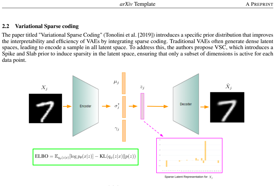
The central object is the spike-probability vector $\gamma = (\gamma_1,\dots,\gamma_d)$ produced by VSC's encoder, where $\gamma_i$ is the probability that latent dimension $i$ is active, i.e., the Bernoulli parameter of the spike variable in a spike-and-slab prior. The paper's new mechanism is a regularizer that, for each class $c$, computes the pairwise Jensen-Shannon distance between the $\gamma$ vectors of samples in that class, averaged over pairs and classes: $\mathcal{L}_{\mathrm{JSD}} = \frac{1}{|C|}\sum_{c\in C}\frac{1}{N_c}\sum_{(k,j)\in c, k\neq j}\sum_{i=1}^d \mathrm{JSD}(\Gamma_{i,k}\|\Gamma_{i,j})$, using the closed-form JSD for Bernoulli distributions. Because the JSD term is bounded and symmetric, it aligns the active dimensions within each class while leaving the VSC sparsity objective intact; the scalar $\lambda$ controls how strongly alignment is enforced.

What would settle it

Train the model with progressively larger $\lambda$ on MNIST and measure (a) the within-class variance of the active-dimension slab values $\mu_i$ and (b) the reconstruction error. The central claim predicts that $\gamma$ vectors converge within a class while slab values retain class-level variety and reconstruction stays bounded; if instead the within-class variance of $\mu_i$ collapses toward zero and reconstruction error rises sharply as $\lambda$ grows, the alignment regularizer is destroying the intra-class variation the paper says it preserves.

Watch

Extended reading notes

Core claim

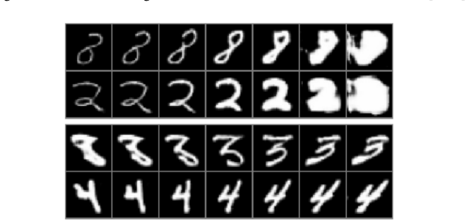
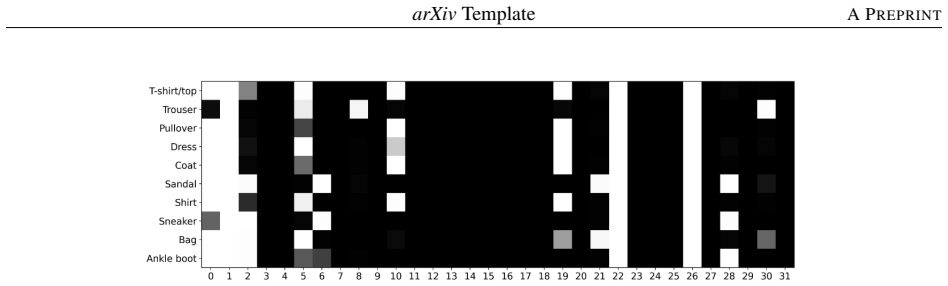
The paper's central claim is that the active dimensions of sparse latent codes should be shared within a class, not chosen per sample. Building on VSC's spike-and-slab prior, where each latent dimension $i$ has a Bernoulli spike variable with success probability $\gamma_i$, the authors propose a loss term $\mathcal{L}_{\mathrm{JSD}}$ that, for each class, averages the Jensen-Shannon distance between the $\gamma$ vectors of every pair of samples in that class. The total objective is $\mathcal{L} = \mathcal{L}_{\mathrm{VSC}} + \lambda \mathcal{L}_{\mathrm{JSD}}$, with the regularizer pushing same-class samples toward the same set of active dimensions. The authors show experimentally that this produces gamma heatmaps with clear per-class masks, and latent traversals reveal that some shared dimensions correspond to global factors (thickness, rotation, vertical contraction) while others correspond to class-specific factors (lower-circle size in digits 3/5/8, heel prominence in shoe classes). They also report that classes within the same category (e.g., boots, sandals, sneakers) have higher Pearson correlation between their average gamma vectors, indicating shared structure at the category level.

Load-bearing premise

The load-bearing assumption is that pushing the per-dimension spike probabilities $\gamma$ of same-class samples toward each other, under the assumption that latent dimensions are independent, is enough to create shared concepts without also collapsing the variation in the non-spike latent values; if the regularizer instead drives every sample in a class to the same $\gamma$ and the same slab values, the 'same attribute, different value' structure is destroyed.

Editorial extensions

If this is right

On datasets where global attributes are ill-defined, the method still yields interpretable class-level factors, which disentanglement methods that assume universal factors cannot.
Latent traversal of a trained model can reveal both global directions (e.g., digit thickness, rotation) and class-specific directions (e.g., stroke intersection in 4/9, heel prominence), giving a vocabulary of concepts per class.
The Pearson correlation between average $\gamma$ vectors of classes can be used to measure category-level similarity, e.g., shoe classes cluster together, which may inform hierarchical or few-shot learning.
The regularizer is a drop-in addition to the VSC objective, so it can be combined with other VAE-based sparse coding variants without architectural changes.

Reading between the lines

Editorial extensions of the paper, not claims the author makes directly.

The same gamma-alignment idea could be applied to spike-and-slab VAEs with different priors or to semi-supervised settings where only a subset of samples has labels, treating the regularizer as a soft clustering constraint.
The paper does not test the effect of $\lambda$ on intra-class slab variance or reconstruction; one natural extension is a scheduled or adaptive $\lambda$ that stops increasing once gamma divergence within a class saturates.
A failure mode worth probing: on classes with high intra-class variation (e.g., a 'dog' class containing many breeds), the regularizer may over-constrain the gamma vectors, forcing the model to either ignore rare sub-structures or compress them into the slab values.
The class-level gamma heatmaps could serve as a post-hoc interpretability tool for supervised classifiers: distilled from a generative model, they give a human-readable mask of which latent factors are used per class.

Share X Bluesky LinkedIn Reddit HN

Editorial analysis

A structured set of objections, weighed in public.

Desk editor's note, referee report, and a circularity audit.

Desk Editor's Note

read the letter

Dear colleague,

Quick take: this is a competent, incremental addition to Variational Sparse Coding. The authors add a within-class Jensen-Shannon regularizer on the spike probabilities gamma, train on MNIST and Fashion-MNIST, and show that class members end up activating the same latent dimensions. That's the whole paper. If you need a sparse VAE with class-aligned activations, this gives you a working recipe plus code.

What's genuine: the JSD closed form for Bernoulli distributions is correct, the algorithm is simple enough to reimplement, and the qualitative results—digit thickness, rotation, garment length, heel prominence—look plausible. I appreciate the appendix with extended traversals and training curves. The class-category observation for Fashion-MNIST (boots/sandals/sneakers share dimensions) is a nice sanity check that the loss induces interpretable grouping.

Soft spots, in order of severity. First, there is a sign inconsistency between Eq. 3 and Eq. 7. Eq. 3 writes the VSC loss as the ELBO (reconstruction plus KL terms); Eq. 7 writes it as the negative of that. The actual optimized objective is therefore unclear. It is probably a typo—the standard VSC loss is the negative ELBO—but it needs fixing before publication.

Second, the evaluation is almost entirely qualitative. There are no quantitative comparisons to VSC or any disentanglement baseline, no reconstruction quality numbers, no sparsity statistics, no error bars across seeds. The central claim—shared dimensions still encode variable attribute values—is asserted but never measured. The stress-test worry that the loss might collapse within-class slab values is real; they should report the dispersion of mu or the z values on shared dimensions for same-class samples.

Third, the class-alignment result is partly circular: the loss directly enforces gamma alignment, so observing alignment is not a surprise. The interesting part is whether the model finds semantically meaningful shared dimensions, and that is supported only by hand-picked traversals from a single run.

None of this is fatal. The method is coherent, the code is promised, and the experiments are reproducible in a weekend. For a workshop or a short conference paper with added quantitative evaluation, it would be a decent fit. As is, I would not let it pass as a full paper: the sign fix and a baseline comparison are mandatory, and the within-class variance analysis is strongly advisable.

Who is this for? Someone building on VSC or using sparse latent models with labeled data. It won't reshape the field, but it's a useful brick. I'd send it to peer review—the core idea is clear and the authors can address the concerns in a revision.

Referee Report

4 major / 5 minor

Summary. This paper extends Variational Sparse Coding (VSC) by adding a class-conditional Jensen-Shannon (JSD) regularizer that encourages samples of the same class to have similar Bernoulli spike probabilities gamma. Equations (4)-(6) define a pairwise within-class JSD term, and Eq. (7) combines it with the VSC objective using a weight lambda. Experiments on MNIST and Fashion-MNIST show average-gamma heatmaps, latent traversals for selected dimensions, and class-pair correlation heatmaps. The central claim is that class-level alignment of active dimensions yields latent spaces where shared dimensions encode interpretable global and class-specific factors, while the values of those factors still vary across samples.

Significance. If the central claim were fully established, the contribution would be a simple and inexpensive modification of VSC that produces class-structured sparse latent spaces, with class-specific interpretability going beyond global disentanglement. The derivation of the closed-form JSD for Bernoulli gamma variables in Eq. (5) is correct, the proposed loss is well specified modulo the sign issue below, and the authors release code. The motivation that classes should share active dimensions while permitting variation in the encoded attribute values is clear, and the Fashion-MNIST category-level correlation results are suggestive. However, the empirical evidence is largely qualitative and lacks quantitative comparison to VSC and disentanglement baselines, repeated-seed variance, or measurements of within-class attribute variation. For these reasons the significance is currently moderate rather than established, and the key claims need additional support.

major comments (4)

[Section 3, Eqs. (3) and (7)] The sign of the VSC loss is inconsistent. Eq. (3) defines L(theta, phi; x_j) with positive signs on the KL-like terms and on the reconstruction term, while Eq. (7) writes L_total with negative signs on the same VSC terms before adding lambda L_JSD. These two expressions differ by an overall sign and by the sign of the reconstruction term. Since Eq. (7) is the objective that is actually minimized, the paper must clarify which expression is optimized and ensure that the reported experiments use the same objective. This issue is load-bearing because the proposed method is defined by this total loss.
[Section 3, Eq. (6); Section 4, Figs. 10 and 17] The headline observation that gamma vectors become aligned within each class is directly enforced by the JSD regularizer, so observing alignment is not independent validation of the method. The paper should provide quantitative evidence that the aligned dimensions correspond to interpretable factors: for example, a comparison with plain VSC using the same architecture, latent dimensionality, and alpha, plus a quantitative interpretability metric or a class-conditional prediction task. Without such evidence, the active-dimension alignment is a consequence of the loss rather than a demonstrated interpretive benefit.
[Section 3 and Section 4.2] The motivating property that class members share active dimensions while still differing in the values of those attributes (Figure 1) is not verified. Because gamma and the slab parameters (mu, sigma) come from the same encoder, the JSD penalty on gamma could in principle also reduce within-class variance of mu on shared dimensions, collapsing the 'same attribute, different value' structure. The paper never reports within-class standard deviation of mu on shared dimensions, nor reconstruction error or negative ELBO of the proposed method versus VSC at matched settings, nor a sweep over lambda. Figures 29 and 39 show that L_JSD decreases and negative ELBO decreases, but they do not establish that within-class attribute variation is preserved.
[Section 4.1 and 4.2] The experimental protocol is too weak to support the central generalization claims. There are no repeated-seed results, no explicit values for alpha, lambda, latent dimension d, or the scheduler mentioned in Appendix A.4, and no numerical comparison to disentanglement baselines beyond qualitative latent traversals reproduced from Chen et al. and Ren et al. The classification of a dimension as 'global' or 'class-specific' is based on visual inspection of heatmaps and selected traversals, with no objective criterion. The paper should add multi-seed quantitative results and specify all hyperparameters and the traversal procedure.

minor comments (5)

[Section 2.2, after Eq. (2)] The sentence 'gamma_i represents the probability of the jth latent variable' should refer to the i-th latent dimension, not the j-th; the same sentence also uses inconsistent indexing.
[Section 3, paragraph after Eq. (6)] The word 'allign' is misspelled and should read 'align'.
[Appendix B.2 heading] The heading 'Fahion-MNIST' is a typo and should read 'Fashion-MNIST'.
[Section 4.2, paragraph after Fig. 16] The phrase 'the 1st and 22th dimensions' should be 'the 1st and 22nd dimensions'.
[General] Latent traversal is the main evaluation tool, but the procedure is not described: which latent samples are used, how far each dimension is changed, and how the traversals are displayed. A precise description would make the qualitative results reproducible.

Circularity Check

1 steps flagged · score 4.0 of 10

Within-class gamma alignment is the optimized objective itself; interpretability claims still rest on independent latent traversals and cross-class metrics.

self definitional [Section 3, Eqs. 6-7; Section 4.1, Figure 10]
"LJSD = 1/|C| sum_{c in C} 1/N_c sum_{(k,j) in c, k != j} JSD(Gamma_j || Gamma_k) ... the proposed term helps to allign the active dimensions for each class of data. As a result, the combination of these two terms ensures that the same latent dimensions are used as much as possible for the data in each class. ... Figure 10: Average gamma probabilities across classes in the MNIST dataset using our proposed method. Active dimensions are well-aligned within each class, improving latent space interpretability."

Equation 6 defines L_JSD as the average pairwise Jensen-Shannon distance between gamma vectors of samples in the same class, and Equation 7 adds this term to the training objective. Minimizing L_total therefore directly drives within-class gamma vectors toward equality. The later observation that active dimensions are 'well aligned within each class' (Figure 10) and that within-class JSD decreases during training (Figures 29 and 39) is a measurement of the optimized objective itself, not an independent consequence of the method. The within-class sharing of active dimensions is enforced by construction; reporting it as an experimental result verifies only that optimization of L_JSD succeeded.

full rationale

No load-bearing self-citations appear: the VSC base (Tonolini et al.) and the Jensen-Shannon distance (Menendez et al.) are external, standard references. The substantive interpretability claims are not fully forced by L_JSD: latent traversals assign post hoc semantics such as thickness, rotation, and heel prominence, and the cross-class Pearson correlations (Figures 15 and 19) are not directly optimized because L_JSD aligns within classes only, not between classes. The sign inconsistency between Eq. 3 and Eq. 7 is a correctness risk, not a circularity. Score 4 reflects one constructed result, within-class gamma alignment being presented as an experimental finding, while the central contribution still retains independent empirical content.

Assumptions & free parameters 2 free parameters · 4 assumptions · 0 invented entities

The central claim leans on the VSC spike-slab model plus a new class-alignment objective with a hand-chosen weight lambda. The main added burden is the assumption that pairwise Bernoulli JSD on gamma is the right alignment signal and that class labels correspond to shared visual attributes. No new entities are introduced.

free parameters (2)

lambda (L_JSD weight) = not reported
Weight of the proposed class-alignment loss in Eq. 7; the appendix says a scheduler gradually increases it, but no schedule values are given. The method's behavior depends on this choice.
alpha (VSC sparsity prior) = not reported
Alpha controls the prior probability that a latent dimension is active in the spike-and-slab prior (Eq. 1). The proposed method inherits it from VSC and the paper gives no value.

assumptions (4)

domain assumption Latent dimensions are independent, so the Jensen-Shannon distance between two samples decomposes into a sum over dimensions.
Invoked in Section 3 before Eq. 4; this independence is inherited from the VSC prior and is used to define the proposed loss.
domain assumption Class labels partition samples according to shared visual attributes that should be encoded by shared active latent dimensions.
Used throughout the method, specifically in Eq. 6 and Algorithm 1; if labels are noisy or semantically incoherent, the regularization pushes gamma vectors toward a meaningless average.
domain assumption The spike variable for each latent dimension follows a Bernoulli distribution parameterized by gamma.
From VSC (Tonolini et al.); used to derive the closed-form JSD in Eq. 5.
standard math The VSC ELBO decomposition in Eq. 2 is correct.
The whole optimization starts from Eq. 2-3; the paper does not re-derive VSC.

how reviews work

0 comments

Cite this review

Pith. "Pith review of Enhancing Interpretability of Sparse Latent Representations with Class Information." pith.science (2026). https://pith.science/paper/GU5DAMCR

@misc{pith2026250514476,
  author       = {Pith},
  title        = {Pith review of: Enhancing Interpretability of Sparse Latent Representations with Class Information},
  year         = {2026},
  howpublished = {\url{https://pith.science/paper/GU5DAMCR}},
  note         = {Machine review of arXiv:2505.14476}
}

read the original abstract

Variational Autoencoders (VAEs) are powerful generative models for learning latent representations. Standard VAEs generate dispersed and unstructured latent spaces by utilizing all dimensions, which limits their interpretability, especially in high-dimensional spaces. To address this challenge, Variational Sparse Coding (VSC) introduces a spike-and-slab prior distribution, resulting in sparse latent representations for each input. These sparse representations, characterized by a limited number of active dimensions, are inherently more interpretable. Despite this advantage, VSC falls short in providing structured interpretations across samples within the same class. Intuitively, samples from the same class are expected to share similar attributes while allowing for variations in those attributes. This expectation should manifest as consistent patterns of active dimensions in their latent representations, but VSC does not enforce such consistency. In this paper, we propose a novel approach to enhance the latent space interpretability by ensuring that the active dimensions in the latent space are consistent across samples within the same class. To achieve this, we introduce a new loss function that encourages samples from the same class to share similar active dimensions. This alignment creates a more structured and interpretable latent space, where each shared dimension corresponds to a high-level concept, or "factor." Unlike existing disentanglement-based methods that primarily focus on global factors shared across all classes, our method captures both global and class-specific factors, thereby enhancing the utility and interpretability of latent representations.

Figures

Figures reproduced from arXiv: 2505.14476 by the authors.

**Figure 1.** Examples of different types of dog ears categorized by shape and structure. This illustrates that within a class [PITH_FULL_IMAGE:figures/full_fig_p003_1.png] view at source ↗

**Figure 2.** VSC architecture. The encoder qϕ(z|x) outputs the mean, standard deviation, and sparsity parameters γ, encouraging sparse latent representations. The decoder pθ(x|z) reconstructs the input. Compared to standard VAEs, VSC promotes interpretability by activating only a subset of latent dimensions. The Spike and Slab prior is defined as: p(z) = Y d i=1 (αN (zi ; 0, 1) + (1 − α)δ(zi)), (1) where δ(.) is the dirac functi… view at source ↗

**Figure 3.** Illustration of global and class-specific factors. Global factors are shared across all classes, while class-specific [PITH_FULL_IMAGE:figures/full_fig_p005_3.png] view at source ↗

Figures from the paper (37 more)

**Figure 4.** Figure 4: Proposed method: aligning active latent dimensions for samples within the same class. For each pair of [PITH_FULL_IMAGE:figures/full_fig_p006_4.png]

**Figure 5.** Figure 5: Calculation of the Jensen-Shannon distance for two samples within the same class. The spike probabilities [PITH_FULL_IMAGE:figures/full_fig_p006_5.png]

**Figure 6.** Figure 6: Computation of the proposed Jensen-Shannon loss term across each class. For each class, the pairwise [PITH_FULL_IMAGE:figures/full_fig_p007_6.png]

**Figure 7.** Figure 7: Average gamma probabilities across classes in the MNIST dataset using VSC. The active latent dimensions [PITH_FULL_IMAGE:figures/full_fig_p009_7.png]

**Figure 8.** Figure 8: Global features discovered in the MNIST dataset using VSC. Left: The twenty-second latent dimension [PITH_FULL_IMAGE:figures/full_fig_p009_8.png]

**Figure 9.** Figure 9: Class-specific features discovered in the MNIST dataset using VSC. Left: The fifth latent dimension may [PITH_FULL_IMAGE:figures/full_fig_p010_9.png]

**Figure 10.** Figure 10: Average gamma probabilities across classes in the MNIST dataset using our proposed method. Active [PITH_FULL_IMAGE:figures/full_fig_p010_10.png]

**Figure 11.** Figure 11: Global features discovered in the MNIST dataset using our proposed method. Left: The second latent [PITH_FULL_IMAGE:figures/full_fig_p010_11.png]

**Figure 12.** Figure 12: Global disentangled features in MNIST obtained from Chen et al. [2016]. [PITH_FULL_IMAGE:figures/full_fig_p011_12.png]

**Figure 13.** Figure 13: Global disentangled features in MNIST obtained from Ren et al. (2021). [PITH_FULL_IMAGE:figures/full_fig_p011_13.png]

**Figure 14.** Figure 14: Class-specific features discovered in the MNIST dataset using our proposed method. Left: The 20th [PITH_FULL_IMAGE:figures/full_fig_p011_14.png]

**Figure 15.** Figure 15: Pearson correlation coefficient between gamma vectors across different MNIST classes using our proposed [PITH_FULL_IMAGE:figures/full_fig_p012_15.png]

**Figure 16.** Figure 16: Average gamma probabilities across classes in the Fashion-MNIST dataset using VSC. Active latent [PITH_FULL_IMAGE:figures/full_fig_p012_16.png]

**Figure 17.** Figure 17: Average gamma probabilities across classes in the Fashion-MNIST dataset using our proposed method. [PITH_FULL_IMAGE:figures/full_fig_p013_17.png]

**Figure 18.** Figure 18: Class-specific interpretations in the Fashion-MNIST dataset using our proposed method. The 10th latent [PITH_FULL_IMAGE:figures/full_fig_p013_18.png]

**Figure 19.** Figure 19: Pearson correlation coefficient between gamma vectors across different Fashion-MNIST classes using our [PITH_FULL_IMAGE:figures/full_fig_p014_19.png]

**Figure 20.** Figure 20: Global feature for the MNIST dataset: The second latent dimension controls digit thickness. [PITH_FULL_IMAGE:figures/full_fig_p016_20.png]

**Figure 21.** Figure 21: Global feature for the MNIST dataset: The eighteenth latent dimension controls rotation along the [PITH_FULL_IMAGE:figures/full_fig_p017_21.png]

**Figure 22.** Figure 22: Global feature for the MNIST dataset: The twenty-second latent dimension controls vertical contraction of [PITH_FULL_IMAGE:figures/full_fig_p018_22.png]

**Figure 23.** Figure 23: Class-specific feature in the MNIST dataset: The sixth latent dimension controls the intersection position for [PITH_FULL_IMAGE:figures/full_fig_p019_23.png]

**Figure 24.** Figure 24: Class-specific feature in the MNIST dataset: The twentieth latent dimension adjusts the lower circle size in [PITH_FULL_IMAGE:figures/full_fig_p019_24.png]

**Figure 25.** Figure 25: Class-specific feature in the MNIST dataset: The seventh latent dimension affects curvature and shape in [PITH_FULL_IMAGE:figures/full_fig_p019_25.png]

**Figure 26.** Figure 26: Pearson correlation coefficient between gamma vectors across different MNIST classes using the proposed [PITH_FULL_IMAGE:figures/full_fig_p020_26.png]

**Figure 27.** Figure 27: Cosine distance between gamma vectors across different MNIST classes using the proposed method. Lower [PITH_FULL_IMAGE:figures/full_fig_p020_27.png]

**Figure 28.** Figure 28: Euclidean distance between gamma vectors across different MNIST classes using the proposed method. [PITH_FULL_IMAGE:figures/full_fig_p021_28.png]

**Figure 29.** Figure 29: Jensen-Shannon divergence between gamma vectors across training epochs for the MNIST dataset, showing [PITH_FULL_IMAGE:figures/full_fig_p021_29.png]

**Figure 30.** Figure 30: -ELBO values across training epochs for the MNIST dataset. [PITH_FULL_IMAGE:figures/full_fig_p022_30.png]

**Figure 31.** Figure 31: Class-specific feature in the Fashion-MNIST dataset: The tenth latent dimension captures garment length in [PITH_FULL_IMAGE:figures/full_fig_p022_31.png]

**Figure 32.** Figure 32: Class-specific feature in the Fashion-MNIST dataset: The nineteenth latent dimension adjusts width or [PITH_FULL_IMAGE:figures/full_fig_p022_32.png]

**Figure 33.** Figure 33: Class-specific feature in the Fashion-MNIST dataset: The twenty-eighth latent dimension controls heel [PITH_FULL_IMAGE:figures/full_fig_p023_33.png]

**Figure 34.** Figure 34: Class-specific feature in the Fashion-MNIST dataset: The thirtieth latent dimension affects the sole thickness [PITH_FULL_IMAGE:figures/full_fig_p023_34.png]

**Figure 35.** Figure 35: Class-specific feature in the Fashion-MNIST dataset: The eighth latent dimension adjusts shape details for [PITH_FULL_IMAGE:figures/full_fig_p023_35.png]

**Figure 36.** Figure 36: Pearson correlation coefficient between gamma vectors across different Fashion-MNIST classes using the [PITH_FULL_IMAGE:figures/full_fig_p024_36.png]

**Figure 37.** Figure 37: Cosine distance between gamma vectors across different Fashion-MNIST classes using the proposed method. [PITH_FULL_IMAGE:figures/full_fig_p024_37.png]

**Figure 38.** Figure 38: Euclidean distance between gamma vectors across different Fashion-MNIST classes using the proposed [PITH_FULL_IMAGE:figures/full_fig_p025_38.png]

**Figure 39.** Figure 39: Jensen-Shannon divergence during training for the Fashion-MNIST dataset. Lower values indicate increased [PITH_FULL_IMAGE:figures/full_fig_p025_39.png]

**Figure 40.** Figure 40: Negative ELBO values during training for the Fashion-MNIST dataset. Lower negative ELBO values [PITH_FULL_IMAGE:figures/full_fig_p026_40.png]

Discussion (0). Sign in to comment.

Reference graph

Works this paper leans on

26 extracted references · 16 canonical work pages

[1]

Selvaraju, Michael Cogswell, Abhishek Das, Ramakrishna Vedantam, Devi Parikh, and Dhruv Batra

Ramprasaath R. Selvaraju, Michael Cogswell, Abhishek Das, Ramakrishna Vedantam, Devi Parikh, and Dhruv Batra. Grad-cam: Visual explanations from deep networks via gradient-based localization. In Proceedings of the IEEE International Conference on Computer Vision, pages 618--626, 2017

2017
[2]

Why should i trust you? explaining the predictions of any classifier

Marco Tulio Ribeiro, Sameer Singh, and Carlos Guestrin. Why should i trust you? explaining the predictions of any classifier. In Proceedings of the 22nd ACM SIGKDD International Conference on Knowledge Discovery and Data Mining, pages 1135--1144, 2016

work page 2016
[3]

A unified approach to interpreting model predictions

Scott Lundberg. A unified approach to interpreting model predictions. arXiv preprint arXiv:1705.07874, 2017

arXiv 2017
[4]

The mnist database of handwritten digits

Yann LeCun. The mnist database of handwritten digits. URL: http://yann.lecun.com/exdb/mnist/. URL https://cir.nii.ac.jp/crid/1571417126193283840

arXiv
[5]

Diederik P. Kingma. Auto-encoding variational bayes. arXiv preprint arXiv:1312.6114, 2013

arXiv 2013
[6]

Generative adversarial networks

Ian Goodfellow, Jean Pouget-Abadie, Mehdi Mirza, Bing Xu, David Warde-Farley, Sherjil Ozair, Aaron Courville, and Yoshua Bengio. Generative adversarial networks. Communications of the ACM, 63 0 (11): 0 139--144, 2020

2020
[7]

Denoising diffusion probabilistic models

Jonathan Ho, Ajay Jain, and Pieter Abbeel. Denoising diffusion probabilistic models. Advances in Neural Information Processing Systems, 33: 0 6840--6851, 2020

2020
[8]

Disentangling disentanglement in variational autoencoders

Emile Mathieu, Tom Rainforth, Nana Siddharth, and Yee Whye Teh. Disentangling disentanglement in variational autoencoders. In International Conference on Machine Learning, pages 4402--4412. PMLR, 2019

work page 2019

Show all 26 references

[9]

Understanding disentangling in beta-vae

Christopher P Burgess, Irina Higgins, Arka Pal, Loic Matthey, Nick Watters, Guillaume Desjardins, and Alexander Lerchner. Understanding disentangling in beta-vae. arXiv preprint arXiv:1804.03599, 2, 2018

2018 arXiv
[10]

Tc-vae: Uncovering out-of-distribution data generative factors

Cristian Meo, Anirudh Goyal, and Justin Dauwels. Tc-vae: Uncovering out-of-distribution data generative factors. arXiv preprint arXiv:2304.04103, 2023

2023 arXiv
[11]

Isolating sources of disentanglement in variational autoencoders

Ricky TQ Chen, Xuechen Li, Roger B Grosse, and David K Duvenaud. Isolating sources of disentanglement in variational autoencoders. Advances in Neural Information Processing Systems, 31, 2018

2018
[12]

Beta-vae: Learning basic visual concepts with a constrained variational framework

Irina Higgins, Loic Matthey, Arka Pal, Christopher P Burgess, Xavier Glorot, Matthew M Botvinick, Shakir Mohamed, and Alexander Lerchner. Beta-vae: Learning basic visual concepts with a constrained variational framework. International Conference on Learning Representations, 3, 2017

2017
[13]

Disentangling by factorizing

Hyunjik Kim and Andriy Mnih. Disentangling by factorizing. In International Conference on Machine Learning, pages 2649--2658. PMLR, 2018

2018
[14]

Discovering interpretable representations for both deep generative and discriminative models

Tameem Adel, Zoubin Ghahramani, and Adrian Weller. Discovering interpretable representations for both deep generative and discriminative models. In International Conference on Machine Learning, pages 50--59. PMLR, 2018

2018
[15]

Infogan: Interpretable representation learning by information maximizing generative adversarial nets

Xi Chen, Yan Duan, Rein Houthooft, John Schulman, Ilya Sutskever, and Pieter Abbeel. Infogan: Interpretable representation learning by information maximizing generative adversarial nets. Advances in Neural Information Processing Systems, 29, 2016

2016
[16]

Unsupervised discovery of interpretable directions in the gan latent space

Andrey Voynov and Artem Babenko. Unsupervised discovery of interpretable directions in the gan latent space. In International Conference on Machine Learning, pages 9786--9796. PMLR, 2020

2020
[17]

Learning disentangled representation by exploiting pretrained generative models: A contrastive learning view

Xuanchi Ren, Tao Yang, Yuwang Wang, and Wenjun Zeng. Learning disentangled representation by exploiting pretrained generative models: A contrastive learning view. arXiv preprint arXiv:2102.10543, 2021

2021 arXiv
[18]

Infogan-cr and modelcentrality: Self-supervised model training and selection for disentangling gans

Zinan Lin, Kiran Thekumparampil, Giulia Fanti, and Sewoong Oh. Infogan-cr and modelcentrality: Self-supervised model training and selection for disentangling gans. In International Conference on Machine Learning, pages 6127--6139. PMLR, 2020

2020
[19]

Glowin: A flow-based invertible generative framework for learning disentangled feature representations in medical images

Aadhithya Sankar, Matthias Keicher, Rami Eisawy, Abhijeet Parida, Franz Pfister, Seong Tae Kim, and Nassir Navab. Glowin: A flow-based invertible generative framework for learning disentangled feature representations in medical images. arXiv preprint arXiv:2103.10868, 2021

2021 arXiv
[20]

A disentangling invertible interpretation network for explaining latent representations

Patrick Esser, Robin Rombach, and Bjorn Ommer. A disentangling invertible interpretation network for explaining latent representations. In Proceedings of the IEEE/CVF Conference on Computer Vision and Pattern Recognition, pages 9223--9232, 2020

2020
[21]

Disdiff: Unsupervised disentanglement of diffusion probabilistic models

Tao Yang, Yuwang Wang, Yan Lv, and Nanning Zheng. Disdiff: Unsupervised disentanglement of diffusion probabilistic models. arXiv preprint arXiv:2301.13721, 2023

2023 arXiv
[22]

Variational sparse coding, 2019

Francesco Tonolini, Bjørn Sand Jensen, and Roderick Murray-Smith. Variational sparse coding, 2019. URL https://openreview.net/forum?id=SkeJ6iR9Km

2019
[23]

Barlow et al

Horace B. Barlow et al. Possible principles underlying the transformation of sensory messages. Sensory Communication, 1 0 (01): 0 217--233, 1961

1961
[24]

Types of dog ears, 2025

A-Z Animals. Types of dog ears, 2025. URL https://a-z-animals.com/pets/dogs/dog-lists/types-of-dog-ears/. Accessed: February 12, 2025

2025
[25]

María Luisa Men \'e ndez, J. A. Pardo, L. Pardo, and M. C. Pardo. The jensen-shannon divergence. Journal of the Franklin Institute, 334 0 (2): 0 307--318, 1997

1997
[26]

H. Xiao. Fashion-mnist: A novel image dataset for benchmarking machine learning algorithms. arXiv preprint arXiv:1708.07747, 2017

2017 arXiv

Pith tools

Reviewed August 7, 2026 · model on record in the stance chip above.

[1] [1]

Selvaraju, Michael Cogswell, Abhishek Das, Ramakrishna Vedantam, Devi Parikh, and Dhruv Batra

Ramprasaath R. Selvaraju, Michael Cogswell, Abhishek Das, Ramakrishna Vedantam, Devi Parikh, and Dhruv Batra. Grad-cam: Visual explanations from deep networks via gradient-based localization. In Proceedings of the IEEE International Conference on Computer Vision, pages 618--626, 2017

2017

[2] [2]

Why should i trust you? explaining the predictions of any classifier

Marco Tulio Ribeiro, Sameer Singh, and Carlos Guestrin. Why should i trust you? explaining the predictions of any classifier. In Proceedings of the 22nd ACM SIGKDD International Conference on Knowledge Discovery and Data Mining, pages 1135--1144, 2016

work page 2016

[3] [3]

A unified approach to interpreting model predictions

Scott Lundberg. A unified approach to interpreting model predictions. arXiv preprint arXiv:1705.07874, 2017

arXiv 2017

[4] [4]

The mnist database of handwritten digits

Yann LeCun. The mnist database of handwritten digits. URL: http://yann.lecun.com/exdb/mnist/. URL https://cir.nii.ac.jp/crid/1571417126193283840

arXiv

[5] [5]

Diederik P. Kingma. Auto-encoding variational bayes. arXiv preprint arXiv:1312.6114, 2013

arXiv 2013

[6] [6]

Generative adversarial networks

Ian Goodfellow, Jean Pouget-Abadie, Mehdi Mirza, Bing Xu, David Warde-Farley, Sherjil Ozair, Aaron Courville, and Yoshua Bengio. Generative adversarial networks. Communications of the ACM, 63 0 (11): 0 139--144, 2020

2020

[7] [7]

Denoising diffusion probabilistic models

Jonathan Ho, Ajay Jain, and Pieter Abbeel. Denoising diffusion probabilistic models. Advances in Neural Information Processing Systems, 33: 0 6840--6851, 2020

2020

[8] [8]

Disentangling disentanglement in variational autoencoders

Emile Mathieu, Tom Rainforth, Nana Siddharth, and Yee Whye Teh. Disentangling disentanglement in variational autoencoders. In International Conference on Machine Learning, pages 4402--4412. PMLR, 2019

work page 2019