Efficient Deconvolution in Populational Inverse Problems
Pith reviewed 2026-05-19 14:16 UTC · model grok-4.3
The pith
A method jointly deconvolves unknown noise and infers parameter distributions from large populations of observations.
A machine-rendered reading of the paper's core claim, the machinery that carries it, and where it could break.
Core claim
The authors establish a methodology for populational inverse problems that simultaneously deconvolves the unknown observational noise distribution and identifies the distribution over model parameters by minimizing a coupled loss function using a modified gradient descent algorithm that exploits noise model structure, combined with an active learning scheme based on adaptive empirical measures for efficient surrogate modeling of parameter-to-solution maps.
What carries the argument
Coupled minimization of a loss over parameter inputs and parameterized observational noise, solved by modified gradient descent leveraging noise structure, plus active learning with adaptive empirical measures for surrogate accuracy in regions of interest.
If this is right
- The approach enables parameter distribution recovery without prior knowledge of the noise distribution.
- It accelerates computation for black-box or expensive physical models through targeted surrogate training.
- It supports automatic differentiation even for nondifferentiable code via the surrogate.
- Applications include porous medium flow, elastodynamics, and atmospheric dynamics models.
Where Pith is reading between the lines
- This joint estimation might generalize to other inverse problems where data comes from repeated experiments under similar conditions.
- Extending the noise parameterization could allow handling more complex noise types like correlated or non-Gaussian without separate calibration.
- Testing on synthetic data with controlled noise would verify if the recovered distributions match the generating ones.
Load-bearing premise
There exists a parameterized form for the observational noise distribution that allows stable joint optimization with the model parameters via the modified gradient descent.
What would settle it
Generate synthetic observations from known parameter distributions and a known noise distribution, then check if the method recovers both distributions to within a small error.
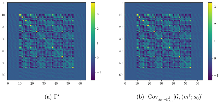
Figures


read the original abstract
This work is focussed on the inversion task of inferring the distribution over parameters of interest leading to multiple sets of observations. The potential to solve such distributional inversion problems is driven by increasing availability of data, but a major roadblock is blind deconvolution, arising when the observational noise distribution is unknown. However, when data originates from collections of physical systems, a population, it is possible to leverage this information to perform deconvolution. To this end, we propose a methodology leveraging large data sets of observations, collected from different instantiations of the same physical processes, to simultaneously deconvolve the data corrupting noise distribution, and to identify the distribution over model parameters defining the physical processes. A parameter-dependent mathematical model of the physical process is employed. A loss function characterizing the match between the observed data and the output of the mathematical model is defined; it is minimized as a function of the both the parameter inputs to the model of the physics and the parameterized observational noise. This coupled problem is addressed with a modified gradient descent algorithm that leverages specific structure in the noise model. Furthermore, a new active learning scheme is proposed, based on adaptive empirical measures, to train a surrogate model to be accurate in parameter regions of interest; this approach accelerates computation and enables automatic differentiation of black-box, potentially nondifferentiable, code computing parameter-to-solution maps. The proposed methodology is demonstrated on porous medium flow, damped elastodynamics, and simplified models of atmospheric dynamics.
Editorial analysis
A structured set of objections, weighed in public.
Referee Report
Summary. The paper proposes a methodology for populational inverse problems that uses large datasets of observations from multiple instantiations of the same physical process to simultaneously deconvolve an unknown observational noise distribution and recover the distribution over model parameters. A parameter-dependent physics model is combined with a loss function that is minimized jointly over the physics parameters and a parameterized noise model via a modified gradient descent algorithm exploiting noise-model structure; an active-learning scheme based on adaptive empirical measures trains a surrogate model for efficiency and enables differentiation of black-box codes. The approach is demonstrated on porous-medium flow, damped elastodynamics, and simplified atmospheric-dynamics models.
Significance. If the joint optimization is stable and the noise parameterization is sufficiently expressive without introducing misspecification bias, the method would provide a practical route to blind deconvolution in settings where population-level data are available, which is relevant to uncertainty quantification and data-driven physics. The surrogate-based active learning component is a clear strength for computational tractability with expensive or nondifferentiable forward maps.
major comments (2)
- [Method] Method description (around the coupled loss minimization): The claim that the modified gradient descent stably solves the joint minimization over physics parameters θ and noise parameters φ rests on the unstated assumptions that the chosen parametric noise family is rich enough to avoid misspecification bias and that the resulting non-convex objective has no spurious local minima that would prevent recovery of the correct (θ, φ) pair. No identifiability analysis, regularization argument, or landscape characterization is supplied to support these conditions for the three physical examples; if either assumption fails, the simultaneous deconvolution and parameter-distribution recovery cannot be guaranteed.
- [Numerical examples] Demonstration sections: The abstract and method outline provide no quantitative error analysis, convergence diagnostics, or ablation on the effect of the noise parameterization choice, making it impossible to verify whether the reported recoveries are robust or sensitive to post-hoc modeling decisions.
minor comments (2)
- [Abstract] Abstract: The phrase 'leverages specific structure in the noise model' is too vague; a brief indication of what structure (e.g., convexity in φ or separability) is exploited would improve clarity.
- [Active learning] The active-learning description would benefit from an explicit statement of how the adaptive empirical measures are updated and how they differ from standard discrepancy-based sampling.
Simulated Author's Rebuttal
We thank the referee for the constructive feedback on our manuscript. We address the major comments point-by-point below, agreeing that additional justification and quantitative support will strengthen the work.
read point-by-point responses
-
Referee: [Method] Method description (around the coupled loss minimization): The claim that the modified gradient descent stably solves the joint minimization over physics parameters θ and noise parameters φ rests on the unstated assumptions that the chosen parametric noise family is rich enough to avoid misspecification bias and that the resulting non-convex objective has no spurious local minima that would prevent recovery of the correct (θ, φ) pair. No identifiability analysis, regularization argument, or landscape characterization is supplied to support these conditions for the three physical examples; if either assumption fails, the simultaneous deconvolution and parameter-distribution recovery cannot be guaranteed.
Authors: We thank the referee for highlighting this important aspect. The current manuscript emphasizes a practical algorithmic framework and its empirical performance on specific physical models rather than providing general theoretical guarantees. We will revise the paper to explicitly articulate the assumptions on the parametric noise family and to include additional numerical experiments (e.g., optimization runs from varied initializations) that probe sensitivity to local minima. A comprehensive identifiability or landscape analysis is model-specific and lies beyond the scope of this work focused on methodology and demonstration. revision: partial
-
Referee: [Numerical examples] Demonstration sections: The abstract and method outline provide no quantitative error analysis, convergence diagnostics, or ablation on the effect of the noise parameterization choice, making it impossible to verify whether the reported recoveries are robust or sensitive to post-hoc modeling decisions.
Authors: We agree that the demonstration sections would benefit from more quantitative support. In the revised manuscript we will add explicit error metrics for recovered distributions, convergence diagnostics for the joint optimization, and an ablation study on noise parameterization choices in at least one example. These additions will improve verifiability of robustness. revision: yes
Circularity Check
No significant circularity; derivation is self-contained
full rationale
The paper defines a joint loss over physics parameters and a parameterized noise model, then minimizes it via a modified gradient descent that exploits noise-model structure, together with an active-learning surrogate based on adaptive empirical measures. None of these steps reduce by construction to fitted inputs renamed as predictions, nor rely on self-citations whose content is itself unverified or load-bearing for the central claim. The methodology is grounded in external observational data from physical processes and standard optimization techniques, with no self-definitional loops or uniqueness theorems imported from the authors' prior work. The derivation therefore remains independent of its own outputs.
Axiom & Free-Parameter Ledger
axioms (2)
- domain assumption Data originates from collections of physical systems instantiating the same underlying processes.
- domain assumption A parameter-dependent mathematical model of the physical process exists and can be evaluated.
Lean theorems connected to this paper
-
IndisputableMonolith/Cost/FunctionalEquation.leanwashburn_uniqueness_aczel unclear?
unclearRelation between the paper passage and the cited Recognition theorem.
We propose a methodology leveraging large data sets of observations... simultaneously deconvolve the data corrupting noise distribution, and to identify the distribution over model parameters... modified gradient descent algorithm that leverages specific structure in the noise model.
-
IndisputableMonolith/Foundation/RealityFromDistinction.leanreality_from_one_distinction unclear?
unclearRelation between the paper passage and the cited Recognition theorem.
L(α,Γ; Γ′) := dy/2 L0(α,Γ; Γ′) + h(α) + r(Γ) ... cut-gradient form
What do these tags mean?
- matches
- The paper's claim is directly supported by a theorem in the formal canon.
- supports
- The theorem supports part of the paper's argument, but the paper may add assumptions or extra steps.
- extends
- The paper goes beyond the formal theorem; the theorem is a base layer rather than the whole result.
- uses
- The paper appears to rely on the theorem as machinery.
- contradicts
- The paper's claim conflicts with a theorem or certificate in the canon.
- unclear
- Pith found a possible connection, but the passage is too broad, indirect, or ambiguous to say the theorem truly supports the claim.
Forward citations
Cited by 3 Pith papers
-
Distributional Inverse Homogenization
Distributional inverse homogenization recovers microstructural statistics from macroscopic mechanical measurements by leveraging collections of bulk data in periodic and stochastic settings.
-
Distributional Inverse Homogenization
Distributional inverse homogenization learns microstructural statistics from bulk mechanical measurements by inverting the homogenization process statistically.
-
Consistency Regularised Gradient Flows for Inverse Problems
A consistency-regularized Euclidean-Wasserstein-2 gradient flow performs joint posterior sampling and prompt optimization in latent space for efficient low-NFE inverse problem solving with diffusion models.
Reference graph
Works this paper leans on
-
[1]
H. W. Engl, M. Hanke, A. Neubauer, Regularization of inverse problems, Vol. 375, Springer Science & Business Media, 1996
work page 1996
- [2]
-
[3]
A. M. Stuart, Inverse problems: a Bayesian perspective, Acta numerica 19 (2010) 451– 559
work page 2010
-
[4]
R. C. Aster, B. Borchers, C. H. Thurber, Parameter estimation and inverse problems, Elsevier, 2018
work page 2018
-
[5]
C. W. Groetsch, C. Groetsch, Inverse problems in the mathematical sciences, Vol. 52, Springer, 1993
work page 1993
- [6]
-
[7]
A. H. Kroese, E. Van der Meulen, K. Poortema, W. Schaafsma, Distributional inference, Statistica Neerlandica 49 (1) (1995) 63–82
work page 1995
-
[8]
D. C. Montgomery, Introduction to statistical quality control, John wiley & sons, 2020
work page 2020
-
[9]
L. A. Bull, P. A. Gardner, J. Gosliga, T. J. Rogers, N. Dervilis, E. J. Cross, E. Pa- patheou, A. Maguire, C. Campos, K. Worden, Foundations of population-based shm, part i: Homogeneous populations and forms, Mechanical systems and signal processing 148 (2021) 107141
work page 2021
-
[10]
T. Schneider, S. Lan, A. Stuart, J. Teixeira, Earth system modeling 2.0: A blueprint for models that learn from observations and targeted high-resolution simulations, Geo- physical Research Letters 44 (24) (2017) 12–396
work page 2017
- [11]
-
[12]
H. Darcy, Les fontaines publiques de la ville de Dijon: exposition et application des principes à suivre et des formules à employer dans les questions de distribution d’eau, Vol. 1, Victor dalmont, 1856
- [13]
-
[14]
M. Alexander, Deconvolution problems in nonparametric statistics, Lecture Notes in Statistics, Springer, Berlin, Heidelberg (2009) 5–138
work page 2009
-
[15]
A. Meister, Deconvolving compactly supported densities, Mathematical Methods of Statistics 16 (2007) 63–76
work page 2007
-
[16]
E. Moulines, J.-F. Cardoso, E. Gassiat, Maximum likelihood for blind separation and deconvolution of noisy signals using mixture models, in: 1997 ieee international confer- ence on acoustics, speech, and signal processing, Vol. 5, IEEE, 1997, pp. 3617–3620
work page 1997
- [17]
-
[18]
E. Oja, A. Hyvarinen, Independent component analysis: algorithms and applications, Neural networks 13 (4-5) (2000) 411–430
work page 2000
-
[19]
A. Hyvärinen, E. Oja, A fast fixed-point algorithm for independent component analysis, Neural computation 9 (7) (1997) 1483–1492
work page 1997
-
[20]
A. Hyvarinen, J. Karhunen, E. Oja, Independent component analysis, Studies in infor- matics and control 11 (2) (2002) 205–207
work page 2002
-
[21]
T.-W. Lee, M. Girolami, T. J. Sejnowski, Independent component analysis using an extended infomax algorithm for mixed subgaussian and supergaussian sources, Neural computation 11 (2) (1999) 417–441
work page 1999
-
[22]
E. Gassiat, S. Le Corff, L. Lehéricy, Deconvolution with unknown noise distribution is possible for multivariate signals, The Annals of Statistics 50 (1) (2022) 303–323
work page 2022
-
[23]
J. Rousseau, C. Scricciolo, Wasserstein convergence in Bayesian and frequentist decon- volution models, The Annals of Statistics 52 (4) (2024) 1691–1715
work page 2024
- [24]
-
[25]
J. Capitao-Miniconi, É. Gassiat, Deconvolution of spherical data corrupted with un- known noise, Electronic Journal of Statistics 17 (1) (2023) 607–649
work page 2023
-
[26]
J. Capitao-Miniconi, É. Gassiat, L. Lehéricy, Deconvolution of repeated measurements corrupted by unknown noise, arXiv preprint arXiv:2409.02014 (2024). 37
-
[27]
J. Johannes, Deconvolution with unknown error distribution, The Annals of Statistics 37 (5A) (2009) 2301 – 2323
work page 2009
- [28]
- [29]
-
[30]
Q. Li, L. Wang, Y. Yang, Differential equation–constrained optimization with stochas- ticity, SIAM/ASA Journal on Uncertainty Quantification 12 (2) (2024) 549–578
work page 2024
- [31]
-
[32]
J. M. Bernardo, A. F. Smith, Bayesian theory, Vol. 405, John Wiley & Sons, 2009
work page 2009
-
[33]
H. Robbins, The empirical bayes approach to statistical decision problems, The Annals of Mathematical Statistics 35 (1) (1964) 1–20
work page 1964
-
[34]
H. E. Robbins, An empirical bayes approach to statistics, in: Breakthroughs in Statis- tics: Foundations and basic theory, Springer, 1992, pp. 388–394
work page 1992
-
[35]
E. Bernton, P. E. Jacob, M. Gerber, C. P. Robert, On parameter estimation with the wasserstein distance, Information and Inference: A Journal of the IMA 8 (4) (2019) 657–676
work page 2019
-
[36]
F. Bassetti, A. Bodini, E. Regazzini, On minimum kantorovich distance estimators, Statistics & probability letters 76 (12) (2006) 1298–1302
work page 2006
- [37]
- [38]
- [39]
-
[40]
D. Bingham, T. Butler, D. Estep, Inverse problems for physics-based process models, Annual Review of Statistics and Its Application 11 (2024)
work page 2024
-
[41]
T. Bui-Thanh, K. Willcox, O. Ghattas, Model reduction for large-scale systems with high-dimensional parametric input space, SIAM Journal on Scientific Computing 30 (6) (2008) 3270–3288. 38
work page 2008
-
[42]
Y. Choi, P. Brown, W. Arrighi, R. Anderson, K. Huynh, Space–time reduced order model for large-scale linear dynamical systems with application to boltzmann transport problems, Journal of Computational Physics 424 (2021) 109845
work page 2021
-
[43]
Z. Bai, Krylov subspace techniques for reduced-order modeling of large-scale dynamical systems, Applied numerical mathematics 43 (1-2) (2002) 9–44
work page 2002
-
[44]
R. W. Freund, Krylov-subspace methods for reduced-order modeling in circuit simula- tion, Journal of Computational and Applied Mathematics 123 (1-2) (2000) 395–421
work page 2000
-
[45]
R. Sampaio, C. Soize, Remarks on the efficiency of pod for model reduction in non-linear dynamics of continuous elastic systems, International Journal for numerical methods in Engineering 72 (1) (2007) 22–45
work page 2007
- [46]
-
[47]
S. Chaturantabut, D. C. Sorensen, Nonlinear model reduction via discrete empirical interpolation, SIAM Journal on Scientific Computing 32 (5) (2010) 2737–2764
work page 2010
-
[48]
B. O. Almroth, P. Stern, F. A. Brogan, Automatic choice of global shape functions in structural analysis, Aiaa Journal 16 (5) (1978) 525–528
work page 1978
-
[49]
A. K. Noor, J. M. Peters, Reduced basis technique for nonlinear analysis of structures, Aiaa journal 18 (4) (1980) 455–462
work page 1980
-
[50]
D. G. Krige, A statistical approach to some basic mine valuation problems on the witwatersrand, Journal of the Southern African Institute of Mining and Metallurgy 52 (6) (1951) 119–139
work page 1951
- [51]
-
[52]
M. C. Kennedy, A. O’Hagan, Bayesian calibration of computer models, Journal of the Royal Statistical Society: Series B (Statistical Methodology) 63 (3) (2001) 425–464
work page 2001
-
[53]
M. C. Kennedy, A. O’Hagan, Predicting the output from a complex computer code when fast approximations are available, Biometrika 87 (1) (2000) 1–13
work page 2000
-
[54]
K. Bhattacharya, B. Hosseini, N. B. Kovachki, A. M. Stuart, Model reduction and neural networks for parametric pdes, The SMAI journal of computational mathematics 7 (2021) 121–157
work page 2021
-
[55]
L. Lu, P. Jin, G. Pang, Z. Zhang, G. E. Karniadakis, Learning nonlinear operators via deeponet based on the universal approximation theorem of operators, Nature machine intelligence 3 (3) (2021) 218–229. 39
work page 2021
-
[56]
N. Kovachki, Z. Li, B. Liu, K. Azizzadenesheli, K. Bhattacharya, A. Stuart, A. Anand- kumar, Neural operator: Learning maps between function spaces with applications to pdes, Journal of Machine Learning Research 24 (89) (2023) 1–97
work page 2023
-
[57]
Z. Li, N. Kovachki, K. Azizzadenesheli, B. Liu, K. Bhattacharya, A. Stuart, A. Anand- kumar, Fourier neural operator for parametric partial differential equations, arXiv preprint arXiv:2010.08895 (2020)
work page internal anchor Pith review Pith/arXiv arXiv 2010
-
[58]
B. Haasdonk, M. Ohlberger, Reduced basis method for finite volume approximationsof parametrizedlinear evolution equations, ESAIM: Mathematical Modelling and Numer- ical Analysis 42 (2) (2008) 277–302
work page 2008
- [59]
-
[60]
L. Yan, T. Zhou, Stein variational gradient descent with local approximations, Com- puter Methods in Applied Mechanics and Engineering 386 (2021) 114087
work page 2021
- [61]
-
[62]
A. Vadeboncoeur, Ö. D. Akyildiz, I. Kazlauskaite, M. Girolami, F. Cirak, Fully prob- abilistic deep models for forward and inverse problems in parametric pdes, Journal of Computational Physics 491 (2023) 112369
work page 2023
-
[63]
Y. Li, Y. Wang, L. Yan, Surrogate modeling for Bayesian inverse problems based on physics-informedneuralnetworks, JournalofComputationalPhysics475(2023)111841
work page 2023
-
[64]
Villani, et al., Optimal transport: old and new, Vol
C. Villani, et al., Optimal transport: old and new, Vol. 338, Springer, 2008
work page 2008
-
[65]
Santambrogio, Optimal transport for applied mathematicians, Vol
F. Santambrogio, Optimal transport for applied mathematicians, Vol. 87, Springer, 2015
work page 2015
-
[66]
N. Bonneel, J. Rabin, G. Peyré, H. Pfister, Sliced and radon wasserstein barycenters of measures, Journal of Mathematical Imaging and Vision 51 (2015) 22–45
work page 2015
-
[67]
A.Gretton, K.M.Borgwardt, M.J.Rasch, B.Schölkopf, A.Smola, Akerneltwo-sample test, The Journal of Machine Learning Research 13 (1) (2012) 723–773
work page 2012
-
[68]
G. J. Székely, M. L. Rizzo, Energy statistics: A class of statistics based on distances, Journal of statistical planning and inference 143 (8) (2013) 1249–1272
work page 2013
-
[69]
G. J. Székely, E-statistics: The energy of statistical samples, Bowling Green State University, Department of Mathematics and Statistics Technical Report 3 (05) (2003) 1–18. 40
work page 2003
-
[70]
M. Rixner, P.-S. Koutsourelakis, A probabilistic generative model for semi-supervised training of coarse-grained surrogates and enforcing physical constraints through virtual observables, Journal of Computational Physics 434 (2021) 110218
work page 2021
-
[71]
Y. Zhu, N. Zabaras, P.-S. Koutsourelakis, P. Perdikaris, Physics-constrained deep learn- ing for high-dimensional surrogate modeling and uncertainty quantification without labeled data, Journal of Computational Physics 394 (2019) 56–81
work page 2019
-
[72]
D. P. Kingma, J. Ba, Adam: A method for stochastic optimization, arXiv preprint arXiv:1412.6980 (2014)
work page internal anchor Pith review Pith/arXiv arXiv 2014
-
[73]
L. Roininen, J. M. J. Huttunen, S. Lasanen, Whittle-matérn priors for Bayesian statis- tical inversion with applications in electrical impedance tomography, Inverse Problems and Imaging 8 (2) (2014) 561–586
work page 2014
-
[74]
M. M. Dunlop, M. A. Iglesias, A. M. Stuart, Hierarchical Bayesian level set inversion, Statistics and Computing 27 (2017) 1555–1584
work page 2017
-
[75]
M. Abramowitz, I. A. Stegun, Handbook of mathematical functions: with formulas, graphs, and mathematical tables, Vol. 55, Courier Corporation, 1965
work page 1965
-
[76]
H. Gottlieb, Eigenvalues of the laplacian with neumann boundary conditions, The ANZIAM Journal 26 (3) (1985) 293–309
work page 1985
- [77]
- [78]
-
[79]
Bleyer, Numerical tours of Computational Mechanics with FEniCSx (Jan
J. Bleyer, Numerical tours of Computational Mechanics with FEniCSx (Jan. 2024)
work page 2024
-
[80]
J. Salençon, Handbook of continuum mechanics: General concepts thermoelasticity, Springer Science & Business Media, 2012
work page 2012
discussion (0)
Sign in with ORCID, Apple, or X to comment. Anyone can read and Pith papers without signing in.