REVIEW 3 major objections 5 minor 7 references
Stochastic Preconditioning for Neural Field Optimization
T0 review · 3 major / 5 minor · reviewed 2026-08-07 · deepseek-v4-flash
Pith's one-line read Adding Gaussian noise to query coordinates makes neural field training behave like optimizing a blurred field, which avoids spurious minima and often beats hand-built coarse-to-fine schemes.
desk verdict A simple, well-tested empirical trick for neural field optimization; the blur framing is loose but the contribution stands. read the letter →
The pith
A machine-rendered reading of the paper's core claim, the machinery that carries it, and where it could break.
The reading
What carries the argument
The load-bearing object is the identity $\operatorname{Blur}_{\alpha}[f](x) = \mathbb{E}_{\varepsilon}[f(x+\varepsilon)]$ with $\varepsilon \sim \mathcal{N}(0,\alpha)$, which turns an intractable convolution over a neural field into a one-line sampling procedure. The method uses a single Monte Carlo sample per query so the computational cost is unchanged, and it adds two practical mechanisms: reflecting perturbed samples across the domain boundary to keep the sampling distribution uniform, and annealing $\alpha$ from an initial scale down to zero so training finishes on the exact unblurred field. An optional extension stores $\alpha(x)$ on a grid and optimizes it through the reparameterization trick, letting the noise scale itself become a learned spatially varying frequency map.
What would settle it
Train the same field and loss on a 2D signal with a known spurious local minimum under three configurations: single-sample Gaussian query noise exactly as proposed, an exact blurred-field loss computed by numerical quadrature or an analytic blur network with the same alpha schedule, and no noise. If the exact blurred loss does not reproduce the improved convergence of the single-sample version, the explanation that stochastic preconditioning optimizes the blurred field is wrong; if no-noise training matches the noisy version, the benefit comes from something other than blur.
Extended reading notes
Core claim
The central claim is that stochastic evaluation is a preconditioner for neural field optimization. If $\varepsilon \sim \mathcal{N}(0,\alpha)$, then $\operatorname{Blur}_{\alpha}[f](x) = \mathbb{E}_{\varepsilon}[f(x+\varepsilon)]$, so replacing every query $x$ by $x+\varepsilon$ during training is, in expectation, querying a blurred low-pass version of the field. The optimizer therefore sees a smoother landscape with fewer spurious local minima, which the paper describes as a stochastic approximation to optimizing through the blurred field. The blur scale starts near two percent of the domain diagonal and is annealed to zero by the first third of training, boundary samples are reflected rather than clamped to preserve a uniform sampling distribution, and a single noisy sample per query is sufficient in the experiments. Across several representations and tasks the paper finds consistent quality gains, and an optional learned spatially varying noise field produces a frequency map of the target signal.
Load-bearing premise
The method assumes that using a single noisy field evaluation through a nonlinear loss, which is a biased estimate of the true blurred-field loss, preserves the optimization benefits of true blurring.
Editorial extensions
If this is right
- Any queryable field, including coordinate MLPs, hashgrids, and triplanes, can obtain coarse-to-fine behavior with one added line of code, giving an immediate quality boost in settings without existing hierarchies.
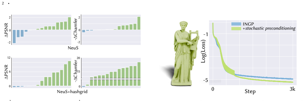
- Hashgrid SDF fitting with stochastic preconditioning reduces Chamfer error dramatically and can make geometric initialization unnecessary, although combining both still works well.
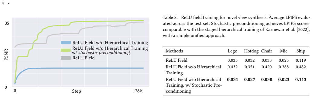
- Removing the custom hierarchy from ReLU fields and using stochastic preconditioning instead produces comparable or better novel-view synthesis quality, at the cost of longer training time because all iterations run at full resolution.
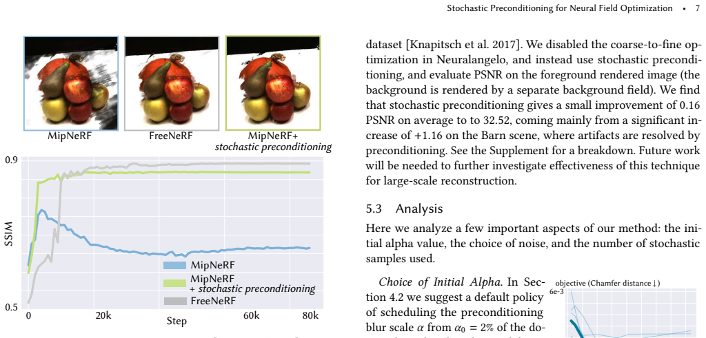
- Sparse-view NeRF training with stochastic preconditioning moves a standard MipNeRF baseline close to a purpose-built frequency-regularization method.
- An optimized spatially varying noise field encodes a level-of-detail map of the target signal and can be used for adaptive sampling and hashgrid feature masking.
Reading between the lines
- One testable extension the paper leaves open is to treat the initial blur scale as a per-region learned quantity from the start, turning the hand-annealed schedule into a fully automatic coarse-to-fine process.
- Because the blur identity is dimension-agnostic, the same query-perturbation trick should apply to non-spatial inputs such as time in dynamic fields or view direction in appearance models, though the paper does not experiment with these.
- The paper's finding that additional samples per query do not help suggests the benefit comes from stochastic gradient smoothing rather than from variance reduction; a direct comparison with deterministic blur would separate these mechanisms.
- If the learned $\alpha$ maps reflect local frequency content, they could be reused outside training, for example to set per-region hashgrid resolutions or to guide mesh extraction, though the paper only demonstrates sampling and feature unlocking.
Editorial analysis
A structured set of objections, weighed in public.
Referee Report
Summary. The paper proposes stochastic preconditioning (SP): during neural field training, query locations are perturbed by Gaussian noise x + eps, eps ~ N(0, alpha), with alpha annealed from an initial value to zero. The method is motivated by the identity Blur_alpha[f](x) = E[f(x + eps)] and is presented as an implicit, stochastic way to optimize through a blurred version of the field. The paper derives boundary handling via reflection, proposes a spatially varying alpha map optimized as an additional parameter, and reports experiments on SDF fitting, surface reconstruction from images, sparse-view NeRF, ReLU fields, and image fitting across several representations. The main claims are that SP improves quality and robustness, matches or outperforms custom hierarchies in several settings, and is simple to integrate, requiring only a few lines of code.
Significance. If the empirical gains hold, the paper describes a genuinely simple and broadly applicable technique that could be adopted across many neural field pipelines. The experimental coverage is extensive, with per-scene tables for DTU, Tanks and Temples, and synthetic NeRF scenes, and the method is tested on coordinate MLPs, hashgrids, triplanes, and ReLU fields. The paper is also admirably honest about its limitations, explicitly acknowledging the bias of single-sample nonlinear loss estimation in Section 6. However, the central theoretical framing is not currently matched to the objective actually optimized: the blur identity applies to field values, while the real losses are nonlinear in the field, so the single-sample procedure is a biased estimator of the blurred-field loss. The paper's own acknowledgment defers analysis, and the single-vs-multiple-samples experiment is too limited to resolve the question. Because the abstract and Section 4 attribute the gains to optimizing through the blurred field, this gap is load-bearing and should be addressed by either additional theoretical analysis or a careful reframing of the claims.
major comments (3)
- [Section 4, Eq. (2), Section 6] The central theoretical justification is not connected to the objective actually optimized. Equation (2) shows E[f_theta(x+epsilon)] = Blur_alpha[f_theta](x) for the field value, but the losses in Sections 5.1 and 5.2 are nonlinear in f_theta, including the SDF loss terms in Eq. (5) and the volumetric rendering loss in Section 5.2. For a quadratic loss, E_epsilon[(f_theta(x+epsilon)-y)^2] = (E[f_theta(x+epsilon)]-y)^2 + Var(f_theta(x+epsilon)), so the single-sample procedure minimizes a biased objective containing a variance penalty, not the blurred-field loss. The paper acknowledges this in Section 6 but only defers analysis ('we do not observe this to cause problems in practice, but there is opportunity for deeper analysis'). Because the abstract and Section 4 attribute the gains to 'querying the blurred field during optimization,' this gap is load-bearing: the empirical improvement could arise from variance regularization, standard input-noise regularization (Bishop 1995), or stochastic gradient noise. I ask for a theoretical analysis of the bias for the concrete losses used, and for experiments that target the mechanism directly, such as comparing single-sample training against training on a multi-sample estimate of E[f] with a matched cumulative query budget.
- [Section 5.3, Table 6] The single-sample versus multiple-samples experiment does not resolve the bias concern. It is run only in the ReLU-field NeRF setting and only up to K=4 samples; for a quadratic loss, K=4 still leaves about one quarter of the variance term, so the comparison does not approach the true blurred-field objective. Moreover, averaging f before the loss reduces but does not eliminate the bias for nonlinear losses, and the reported PSNR differences (33.72, 33.74, 33.79) are small and likely within noise. A convincing control would use a larger K, or a closed-form estimate of E[f], and confirm whether the benefits of stochastic preconditioning persist when the variance bias is suppressed.
- [Section 5.2 vs. Supplement Table 5] The main text states that stochastic preconditioning yields 'high quality results on-par with FreeNeRF' in the sparse-view NeRF setting, and the abstract claims matching or outperforming custom-designed hierarchies, but Supplement Table 5 shows that MipNeRF with stochastic preconditioning generally underperforms FreeNeRF on the reported scenes (e.g., 0.582 vs. 0.698 on scene 21, 0.699 vs. 0.746 on scene 55, 0.758 vs. 0.812 on scene 103). The supplement itself states 'Stochastic preconditioning improves upon the baseline but generally underperforms FreeNeRF.' The comparative claims in the main text and abstract should be revised to reflect the full results, and the settings in which the method matches, exceeds, or falls short should be stated explicitly.
minor comments (5)
- [Section 5.1.2] The phrase 'See Table 2 and Table 3 for full tables in the supplemental document' is confusing because the main text already contains a Table 2; renumber or rename the supplement tables to avoid ambiguity.
- [Supplement A.1.3] The text says 'Please see Section A.1.3 in main paper' but the discussion of fully-supervised SDF fitting is in the supplement; correct the cross-reference.
- [Figure 1] The label 'Ground Truth α-Map' is misleading because the optimized alpha map is not a ground-truth frequency map; consider using 'Optimized α-Map' instead.
- [Section 3.2] The loss-landscape inset is presented as qualitative evidence of more isotropic level sets; this is fine as intuition but should be explicitly labeled as illustrative rather than a quantitative conditioning analysis.
- [Section 5.2] Figure 8 reports PSNR values in the figure but not in a table; adding a small table with per-scene PSNR/LPIPS numbers would improve reproducibility and readability.
Circularity Check
No significant circularity: the core blur-expectation identity is standard, and all improvement claims are evaluated against external baselines with free hyperparameters.
full rationale
The paper's derivation chain is self-contained and does not reduce to its own inputs. The key identity, Blur[f](x) = E[f(x + eps)] with eps ~ N(0, alpha) (Eq. 2), is a standard Monte Carlo / Gaussian-smoothing fact, not an author-derived result, and it is not used to define the target metric. The central empirical claims are comparisons against unmodified external baselines (NeuS, Neuralangelo, FreeNeRF, ReLU fields, INGP, MipNeRF), so the reported improvements are not forced by construction. The alpha schedule is a free hyperparameter selected experimentally in Section 5.3, but the paper's headline result is not a prediction of a quantity that alpha was fitted to reproduce. The Section 6 statement that 'sampling a nonlinear loss function with a single sample is a biased estimator for the loss on the true blurred field' is an explicit, honest limitation; it identifies a mismatch between the motivating identity and the actual optimized objective, which is a correctness or interpretation risk rather than a circular dependency. No load-bearing self-citation appears: citations to author-affiliated work are contextual (e.g., Takikawa et al. 2023a) and do not justify the core claim. The spatially-varying alpha map in Section 5.5 is an optimized quantity whose interpretation as a frequency map is post-hoc, but it is not presented as an independent prediction of ground-truth content. Overall, the paper's contributions are measured against external benchmarks and do not collapse into a fit or a self-citation chain.
Assumptions & free parameters
free parameters (3)
- initial blur scale alpha0 =
0.02 (point clouds), 0.013 (NeuS), 0.03 (Neuralangelo), 0.04 (MipNeRF), 0.003 (ReLU fields)
- alpha annealing schedule =
exponential to 0 at 1/3 of training, or single-step after 2000 steps in some experiments
- spatially varying alpha grid resolution and learning rate =
128x128x128 grid with lr 1e-3 for Neuralangelo; image/16 grid with lr 0.01 for images
assumptions (5)
- standard math Gaussian blur of a signal equals convolution with a Gaussian kernel, and can be expressed as an expectation over Gaussian perturbations (Eq 1-2).
- domain assumption A single Monte Carlo sample provides a usable gradient estimate for the blurred field objective.
- domain assumption Reflecting perturbed samples at domain boundaries preserves the desired sampling distribution.
- ad hoc to paper Annealing alpha from a large value to zero yields coarse-to-fine optimization benefits.
- domain assumption Blurring the field during optimization eases escape from poor local minima.
Cite this review
Pith. "Pith review of Stochastic Preconditioning for Neural Field Optimization." pith.science (2026). https://pith.science/paper/AQA3UWK7
@misc{pith2026250520473,
  author       = {Pith},
  title        = {Pith review of: Stochastic Preconditioning for Neural Field Optimization},
  year         = {2026},
  howpublished = {\url{https://pith.science/paper/AQA3UWK7}},
  note         = {Machine review of arXiv:2505.20473}
}
read the original abstract
Neural fields are a highly effective representation across visual computing. This work observes that fitting these fields is greatly improved by incorporating spatial stochasticity during training, and that this simple technique can replace or even outperform custom-designed hierarchies and frequency space constructions. The approach is formalized as implicitly operating on a blurred version of the field, evaluated in-expectation by sampling with Gaussian-distributed offsets. Querying the blurred field during optimization greatly improves convergence and robustness, akin to the role of preconditioners in numerical linear algebra. This implicit, sampling-based perspective fits naturally into the neural field paradigm, comes at no additional cost, and is extremely simple to implement. We describe the basic theory of this technique, including details such as handling boundary conditions, and extending to a spatially-varying blur. Experiments demonstrate this approach on representations including coordinate MLPs, neural hashgrids, triplanes, and more, across tasks including surface reconstruction and radiance fields. In settings where custom-designed hierarchies have already been developed, stochastic preconditioning nearly matches or improves their performance with a simple and unified approach; in settings without existing hierarchies it provides an immediate boost to quality and robustness.
Figures


Figures from the paper (11 more)





Reference graph
Works this paper leans on
-
[5]
ACM transactions on graphics (TOG) 41, 4 (2022), 1–15
Instant neural graphics primitives with a multiresolution hash encoding. ACM transactions on graphics (TOG) 41, 4 (2022), 1–15. Vincent Sitzmann, Julien Martel, Alexander Bergman, David Lindell, and Gordon Wetzstein
work page 2022
-
[1987]
Marching cubes: A high resolution 3D surface construction algorithm. SIGGRAPH Comput. Graph. 21, 4 (Aug. 1987), 163–169. https://doi.org/10.1145/37402.37422 Thomas Müller
arXiv 1987
-
[2014]
arXiv preprint arXiv:1412.6980 (2014)
Adam: A method for stochastic optimization. arXiv preprint arXiv:1412.6980 (2014). Arno Knapitsch, Jaesik Park, Qian-Yi Zhou, and Vladlen Koltun
arXiv 2014
-
[2017]
ACM Transactions on Graphics (ToG) 36, 4 (2017), 1–13
Tanks and temples: Benchmarking large-scale scene reconstruction. ACM Transactions on Graphics (ToG) 36, 4 (2017), 1–13. Zhaoshuo Li, Thomas Müller, Alex Evans, Russell H Taylor, Mathias Unberath, Ming- Yu Liu, and Chen-Hsuan Lin
work page 2017
-
[2020]
Advances in neural information processing systems 33 (2020), 7462–7473
Implicit neural representations with periodic activation functions. Advances in neural information processing systems 33 (2020), 7462–7473. Peng Wang, Lingjie Liu, Yuan Liu, Christian Theobalt, Taku Komura, and Wenping Wang
work page 2020
-
[2021]
arXiv preprint arXiv:2106.10689 (2021)
Neus: Learning neural implicit surfaces by volume rendering for multi-view reconstruction. arXiv preprint arXiv:2106.10689 (2021). Yiqun Wang, Ivan Skorokhodov, and Peter Wonka
arXiv 2021
-
[2022]
In ACM SIGGRAPH 2022 conference proceedings
Relu /f_ields: The little non-linearity that could. In ACM SIGGRAPH 2022 conference proceedings . 1–9. Diederik P Kingma
work page 2022
Reviewed August 7, 2026 · model on record in the stance chip above.
Discussion (0). Continue with ORCID to comment.