REVIEW 3 major objections 6 minor 46 references
Generating Hypotheses of Dynamic Causal Graphs in Neuroscience: Leveraging Generative Factor Models of Observed Time Series
T0 review · 3 major / 6 minor · reviewed 2026-08-07 · deepseek-v4-flash
Pith's one-line read Dynamic causal graphs in time series can be recovered as behavior-weighted mixtures of a few static nonlinear factor graphs, and the REDCLIFF-S model recovers them with 22–28% higher F1 scores than baselines on synthetic benchmarks.
desk verdict A genuinely new dynamic-graph factor model with honest limitations; the synthetic wins are real but in-distribution, and the paper oversells the no-assumption framing. read the letter →
The pith
A machine-rendered reading of the paper's core claim, the machinery that carries it, and where it could break.
The reading
What carries the argument
The load-bearing identity is the conditionally weighted superposition $\Phi(t) = G(t) \odot^\dagger F(t) = \sum_k G(t)_k F_k(t)$, where $\odot^\dagger$ denotes broadcast multiplication of the score vector $G(t)$ against the tensor of factor outputs. The identity splits estimation into two tasks: each factor $f_{\phi_k}$ is a cMLP whose first-layer weights are time-lagged adjacency matrices $\hat{A}_{:,:,t}$, so a factor literally is an inspectable causal graph; and the state model $g_\theta$ maps a longer history window to nonnegative scores, deciding which factor dominates at each time step. A cosine-similarity penalty between factor graphs enforces the prior that factors should serve different purposes, and in REDCLIFF-S an invertible map lets a subset of scores double as predicted behavioral labels, so the factorization carries the hypothesis directly.
What would settle it
Run the method on a system whose causal edge strengths drift continuously through many values rather than switching between a few patterns; if REDCLIFF-S's fixed factors cannot track the drift at better than static-baseline accuracy, the superposition model is the reason. A sharper test is the paper's own two-node counterexample, in which ReLU and nReLU edges become observationally equivalent: Appendix A.1 argues no method can identify which state generated a sample, and verifying empirically that REDCLIFF-S assigns such samples at chance level would confirm the stated limit rather than a recoverable signal.
Extended reading notes
Core claim
REDCLIFF-S claims that a dynamic causal graph can be modeled as $\Phi(t) = \sum_{k=1}^{K} G(t)_k F_k(t)$: a small number of static factor functions $F_k$, each mapping past variable values to present values and each yielding an explicit time-lagged adjacency matrix of Granger causal weights, combined by history-conditioned scores $G(t)$ produced by a state model $g_\theta$. Because each factor is a component-wise MLP, the relationships inside a factor can be nonlinear, and because the scores vary with time, the composite graph can change direction and strength without assuming a discrete switch between states. In the supervised variant, behavioral labels are attached to particular factor scores through invertible maps, so each factor's adjacency matrix can be read as the candidate wiring hypothesis for that behavior. The paper reports that this construction outperforms static nonlinear, dynamic-linear, and regime-switching baselines in F1 and ROC-AUC on synthetic data and on D4IC, a five-fold mixture version of DREAM4, and it demonstrates factor graphs for Open Field, Home Cage, Tail Suspension, and Social Preference states that reproduce published findings such as lateral habenula involvement in stress.
Load-bearing premise
The recorded system must actually be expressible as a small set of reusable interaction patterns whose relative importance at each moment is set by recent history; if the true interactions instead morph continuously into new forms, the factor graphs and scores have no faithful target to recover.
Editorial extensions
If this is right
- Each trained factor yields a fixed, inspectable adjacency matrix, so a REDCLIFF-S run outputs concrete candidate edges, with direction, lag, and strength, that can seed interventional studies such as dynamic causal models.
- Attaching behavioral labels to factor scores means the output includes a wiring diagram per behavior rather than one averaged graph; on the TST data this produces distinct Open Field, Home Cage, and Tail Suspension hypotheses from a single training run.
- Because factors are nonlinear, the approach beats linear dynamic factor models on systems with ReLU and nReLU edges, where the ground truth is unrepresentable by any linear model.
- The ablation results attribute most of the gain to multiple factors, learned scores, and the supervised term, while the cosine-similarity penalty helps on sparse systems and can be dropped on dense ones.
- The authors' non-identifiability proof implies that no method of this family can uniquely recover true factor graphs in general, so the practical claim is narrower: the recovered graphs are useful hypotheses even when not unique.
Reading between the lines
- If real neural dynamics only approximate the superposition assumption, factor graphs may still serve as a low-dimensional grammar of the dominant interaction modes, with the scores acting as a behavioral readout; under misspecification the model would remain a dimension-reduction tool rather than an exact recovery method.
- The cosine-similarity penalty is a proxy for functional dissimilarity of graphs, and a testable extension would replace it with a sparsity prior on factor usage to check whether rare behavioral states are recovered better.
- The TST hypothesis that the anterior-lateral habenula drives several regions in the stressful Open Field condition is directly interventional: silencing the lateral habenula during tail suspension would test whether that edge carries causal weight.
- Because the model needs no interventional data and accepts any scalar time series with global state labels, it could transfer to sleep staging, anesthesia depth monitoring, or economic regime detection, wherever states mark distinct dynamics.
Editorial analysis
A structured set of objections, weighed in public.
Referee Report
Summary. The paper proposes REDCLIFF-S, a factor-based Granger causal discovery method that models dynamic causal graphs as a history-conditioned weighted sum of static factor graphs, with each factor implemented as a cMLP and regularized for sparsity and factor dissimilarity; optional supervised labels are included through an invertible state model. The authors claim substantial improvements over static and linear baselines in detecting nonlinear, state-dependent causal interactions, based on synthetic benchmarks (Synthetic Systems and D4IC) and two real-world LFP case studies (TST and Social Preference). The paper also releases code and reports standard errors and ROC-AUC values alongside F1 scores.
Significance. If the central claims were fully supported, this would be a useful contribution to hypothesis generation in neuroscience: the method is explicitly designed for interpretability (fixed factor graphs, behavior-linked factor scores), combines nonlinear factors with dynamic weighting in a natural way, and is evaluated against multiple baselines with released code and standard errors. The design principle of reusable factor graphs with state-dependent weights is plausible, and the in-distribution synthetic results are encouraging. However, as detailed below, the external validity of the evaluation and the consistency between the paper's identifiability analysis and its benchmark design require substantial work before the abstract's claims about detecting complex, time-varying interactions can be accepted.
major comments (3)
- [Section 4.1 and Eq. (4)] The synthetic evaluation is in-distribution for the model class. Section 4.1 generates each recording as a time-varying weighted superposition of VAR models with ReLU/nReLU edges, exactly the form of Eq. (4), and Section 4.3 constructs D4IC by the same mixing mechanism over DREAM4 folds. The Section 1 statement that 'we make no assumptions regarding the underlying generative processes' is therefore contradicted by both the model form and the evaluation design. Because the real-data case studies in Section 5 lack ground truth, the paper provides no evidence for performance when the true dynamics are not a small weighted superposition of reused static graphs. Please add experiments where the target system is outside the model class (e.g., continuously morphing edge weights, or edge functions that change form over time) or substantially soften the no-assumptions claim and the abstract's characterization of what is supported.
- [Appendix A.1 and Section 4.1] The paper's own identifiability result directly weakens the benchmark's validity. Appendix A.1 proves that a two-node system with ReLU and nReLU edges and symmetric innovations has two observationally equivalent state-dependent graphs, and Section 4.1 explicitly uses ReLU and nReLU activations in the synthetic systems. The same sign/flip symmetry may therefore be present in the synthetic ground truth, which would mean that edge-level F1 and ROC-AUC scores in Section 4.2 and Tables 2, 5, and 6 penalize algorithms for recovering observationally equivalent alternatives. Please either establish that the synthetic data generation avoids the A.1 symmetry (e.g., via asymmetric innovation distributions or initial conditions), or evaluate against equivalence classes rather than a single ground-truth graph; at minimum, the relationship between A.1 and the benchmark's ground truth should be discussed explicitly.
- [Section 3.5 and Section 5] The behavioral link is partly imposed by the supervised construction and should not be described as an emergent discovery. In Eq. (8), the first B factor weights are assigned to behavioral labels, and Eq. (9) trains the state model to predict those labels through the lambda*MSE term. Consequently, the finding that specific factors 'correspond' to Open Field or Home Cage states in the TST case study reflects the imposed supervised structure as much as an independent property of the data. The real-data analysis should be framed as hypothesis generation with the caveat that the behavior-factor association is built into the loss, and the authors should provide a corresponding unsupervised or held-out validation to support the claim of uncovering behavior-linked relationships.
minor comments (6)
- [Abstract and Appendix C.1] The phrase 'in some of our experiments' makes the headline improvement of 22-28% (and 'well over 60%') untestable; please cite the specific systems and figure numbers (e.g., Figure 6 and Supplementary Figure 9) in the abstract or clarify the qualifier in the main text.
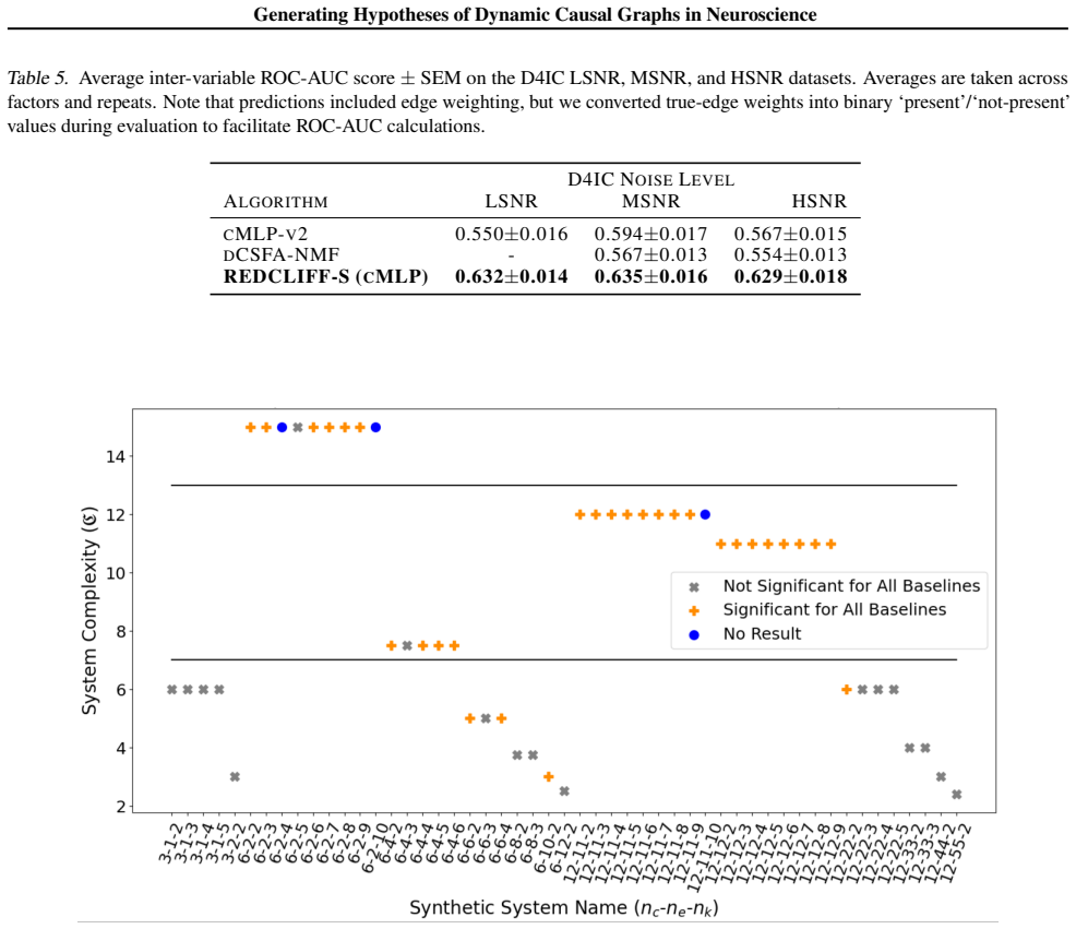
- [Section 4.2] The system naming convention '6-2-2', '6-4-2', '12-11-2', '12-11-5' is not defined; please state at first use that the triple denotes (number of nodes, number of inter-variable edges, number of factors).
- [Table 3 and Appendix C.6] The up/down arrows in Table 3 are ambiguous because the baseline for comparison is not specified; please state that arrows indicate change relative to the full REDCLIFF-S model, and note that for the two systems where the rho=0 ablation improves performance, this should be acknowledged in the main text discussion of the cosine-similarity penalty.
- [Figure 5] The color scale for 'difference in mean normalized causal estimates' is not defined; please describe how the normalization and difference are computed, since the figure is the primary evidence for the TST case study.
- [Appendix A.2.2] The proof sketch of Lemma 1 is difficult to follow: the notation p(f_i, X) is used in a way that conflates a joint density and a conditional likelihood, and the step from Eq. (13) to Eq. (14) relies on the uniform-state prior in a way that should be stated explicitly; please rewrite the derivation for clarity.
- [General] There are minor typographical and formatting issues, including 'it's use' in Section 4.3, inconsistent 'Open Field (OP)' vs 'OF' in Appendix D.1 and Section 5, and the unexpanded 'V AR' spacing in several places.
Circularity Check
All synthetic benchmarks generate the true system inside the model's own Eq. 4 superposition class, so the paper's central structural assumption is never tested; the behavior-linked factors in the TST case study are partly imposed by the supervised loss of Eq. 9.
-
self definitional
[Section 3.1 (Problem Statement); Section 3.2/Eq. 4; Section 4.1 (Synthetic Data Generation); Section 4.3 (D4IC)]
"Indeed, in Sections 4.1, 4.2, and 4.3 we implement Φ as a factor model itself (see Section 3.2 for formalization). ... Recordings obtained from each VAR model were then weighted over time with linearly interpolated weights (randomly selected between 0 and 1). These weighted recordings were added together along with a level of Gaussian noise."
The benchmarks define the target system by the model's own hypothesis. Eq. 4 sets REDCLIFF's form as Φ(t) = Σ_k G(t)_k F_k(t), and Section 3.1 states that in all experiments 'we implement Φ as a factor model itself': each synthetic system is a set of fixed VAR factors combined by time-varying scalar weights ('weighted over time with linearly interpolated weights... added together'), and D4IC likewise superposes DREAM4 folds by adding down-weighted recordings. Hence every ground-truth graph the method is tested on is, by construction, a small weighted sum of reused static factor graphs — exactly the class the model assumes.
-
fitted input called prediction
[Section 3.5 (REDCLIFF-S, Eqs. 8-9, λ=100 in Tables 19-20); Section 5 (TST case study, Figure 5)]
"Thus, we follow prior literature and assign behaviors to the first B elements of α (Mague et al., 2022) ... we add a supervised component to L in Eq. 7 to obtain L(ϕ, θ,D) = Lf (ϕ, D) + Lg(θ, D) + λMSE(Y, Ŷ) (9) ... In Figure 5 we show the difference between mean normalized causal estimates for the REDCLIFF-S factors assigned to the Open Field (OF) and Home Cage (HC) behavioral paradigms."
The factor-behavior coupling is imposed by the loss, then reported as a discovery. Eq. 9 supervises the first B factor scores to reproduce the behavioral labels (λ = 100), and Eq. 8 defines the predicted label as an invertible function of exactly those scores, ŷ = gy(gα^{-1}(α:B)). The TST case study then presents the difference between 'REDCLIFF-S factors assigned to the Open Field (OF) and Home Cage (HC) behavioral paradigms' as evidence of behavior-linked causal structure. Under Eq. 9, factors are forced to track the behavioral states during training, so the finding that the OF factor differs from the HC factor is partly guaranteed by construction; only the edge weights inside each factor are genuinely learned from the forecasting objective.
full rationale
The paper's principal empirical claims — roughly 22-28% mean optimal-f1 improvements over static/linear baselines on Synthetic Systems and D4IC — are anchored to externally defined ground-truth graphs and external baselines, so they are not fabricated by fitting. The model genuinely learns nontrivial quantities: recovered accuracy varies with complexity and SNR (ROC-AUC 0.63-0.80; ablations degrade performance), and the baselines are independent implementations. However, the method's central structural premise — that real dynamics are a small weighted superposition of reused static factor graphs (Eq. 4) — is never stress-tested: Section 3.1 states that in all experiments 'we implement Φ as a factor model itself,' with VAR factors and linearly interpolated weights, so the Synthetic Systems and D4IC ground truths are generated inside the model's own hypothesis class. This is compounded by the supervised construction of Eqs. 8-9, where behaviors are assigned to the first B factor scores and used as training targets, so the behavior-linked factor separation in the TST case study is in part imposed by the objective rather than discovered. Real-data corroboration also leans partly on same-group prior work (Talbot et al., 2023; Mague et al., 2022), but the synthetic comparisons do not depend on those citations, so self-citation is not load-bearing for the main result. Net: partial circularity concentrated in the self-definitional benchmarks and the supervised factor-behavior coupling; score 4.
Assumptions & free parameters
free parameters (5)
- Loss coefficients eta, omega, rho, gamma, lambda =
omega=10.0; rho=1/sum(i); gamma=0.001; lambda=100.0; eta=0.1/(nk*sqrt(nc^2-1))
- Number of factors nk =
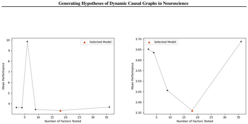
Set equal to dataset B for synthetic and D4IC; nk=9 for TST; nk in [2,4,6,9,18,36] for SP
- State-model context length tau_cl (embedded lag tau_in + tau_cl) =
16 for synthetic and real datasets; 20 for D4IC
- Behavioral presence threshold c_b =
Not specified in the paper
- Input lag order tau_in for generative factors =
4 for REDCLIFF-S experiments; 2 for synthetic system generation
assumptions (5)
- domain assumption The observed time series are generated by a system Phi(t) that is exactly a finite weighted superposition of K* static factor functions F_k with weights G(t), as in Section 3.2 and Equation 4.
- domain assumption The first-layer weights of each cMLP factor faithfully represent Granger causal relationships between variables.
- domain assumption Global state or behavioral labels are available and correspond to one dominant generative factor at each time step.
- domain assumption Cosine similarity between estimated factor graphs is a useful proxy for graph dissimilarity and for model selection and stopping.
- domain assumption A dynamic causal graph can be fairly summarized by lag-summed adjacency matrices and binary thresholded edges for evaluation.
Cite this review
Pith. "Pith review of Generating Hypotheses of Dynamic Causal Graphs in Neuroscience: Leveraging Generative Factor Models of Observed Time Series." pith.science (2026). https://pith.science/paper/ZALQ7YU2
@misc{pith2026250520697,
  author       = {Pith},
  title        = {Pith review of: Generating Hypotheses of Dynamic Causal Graphs in Neuroscience: Leveraging Generative Factor Models of Observed Time Series},
  year         = {2026},
  howpublished = {\url{https://pith.science/paper/ZALQ7YU2}},
  note         = {Machine review of arXiv:2505.20697}
}
read the original abstract
The field of hypothesis generation promises to reduce costs in neuroscience by narrowing the range of interventional studies needed to study various phenomena. Existing machine learning methods can generate scientific hypotheses from complex datasets, but many approaches assume causal relationships are static over time, limiting their applicability to systems with dynamic, state-dependent behavior, such as the brain. While some techniques attempt dynamic causal discovery through factor models, they often restrict relationships to linear patterns or impose other simplifying assumptions. We propose a novel method that models dynamic graphs as a conditionally weighted superposition of static graphs, where each static graph can capture nonlinear relationships. This approach enables the detection of complex, time-varying interactions between variables beyond linear limitations. Our method improves f1-scores of predicted dynamic causal patterns by roughly 22-28% on average over baselines in some of our experiments, with some improvements reaching well over 60%. A case study on real brain data demonstrates our method's ability to uncover relationships linked to specific behavioral states, offering valuable insights into neural dynamics.
Figures


Figures from the paper (19 more)






Reference graph
Works this paper leans on
-
[1]
write newline
" write newline "" before.all 'output.state := FUNCTION n.dashify 't := "" t empty not t #1 #1 substring "-" = t #1 #2 substring "--" = not "--" * t #2 global.max substring 't := t #1 #1 substring "-" = "-" * t #2 global.max substring 't := while if t #1 #1 substring * t #2 global.max substring 't := if while FUNCTION format.date year duplicate empty "emp...
-
[2]
Allen, E. A., Liu, J., Kiehl, K. A., Gelernter, J., Pearlson, G. D., Perrone-Bizzozero, N. I., and Calhoun, V. D. Components of cross-frequency modulation in health and disease. Frontiers in systems neuroscience, 5: 0 59, 2011
work page 2011
-
[3]
K., Devijver, E., and Gaussier, E
Assaad, C. K., Devijver, E., and Gaussier, E. Survey and evaluation of causal discovery methods for time series. Journal of Artificial Intelligence Research, 73: 0 767--819, 2022
2022
-
[4]
Causal discovery from conditionally stationary time series
Balsells-Rodas, C., Tu, R., Li, Y., and Kjellstrom, H. Causal discovery from conditionally stationary time series. In UAI 2022 Workshop on Causal Representation Learning, 2022
work page 2022
-
[5]
Neural additive vector autoregression models for causal discovery in time series
Bussmann, B., Nys, J., and Latr \'e , S. Neural additive vector autoregression models for causal discovery in time series. In Discovery Science: 24th International Conference, DS 2021, Halifax, NS, Canada, October 11--13, 2021, Proceedings 24, pp.\ 446--460. Springer, 2021
work page 2021
-
[6]
D., Miller, R., Pearlson, G., and Adal , T
Calhoun, V. D., Miller, R., Pearlson, G., and Adal , T. The chronnectome: time-varying connectivity networks as the next frontier in fmri data discovery. Neuron, 84 0 (2): 0 262--274, 2014
work page 2014
-
[7]
Multi-region local field potential recordings during a tail-suspension test
Carlson, D., Kumar, S., and Dzirasa, K. Multi-region local field potential recordings during a tail-suspension test. Duke Research Data Repository, 2023
work page 2023
-
[8]
Dycast: learning dynamic causal structure from time series
Cheng, Y., Lyu, B., Xing, W., and Zhu, Z. Dycast: learning dynamic causal structure from time series. 2025
work page 2025
Show all 46 references
-
[9]
Multiscale causal structure learning
D'Acunto, G., Di Lorenzo, P., and Barbarossa, S. Multiscale causal structure learning. arXiv preprint arXiv:2207.07908, 2022
2022 arXiv
-
[10]
M., Kumar, S., Dancy, E
Dzirasa, K., Coque, L., Sidor, M. M., Kumar, S., Dancy, E. A., Takahashi, J. S., McClung, C. A., and Nicolelis, M. A. Lithium ameliorates nucleus accumbens phase-signaling dysfunction in a genetic mouse model of mania. Journal of Neuroscience, 30 0 (48): 0 16314--16323, 2010
2010
-
[11]
B., Jordan, M
Fox, E., Sudderth, E. B., Jordan, M. I., and Willsky, A. S. Bayesian nonparametric inference of switching dynamic linear models. IEEE Transactions on signal processing, 59 0 (4): 0 1569--1585, 2011
2011
-
[12]
Friston, K., Moran, R., and Seth, A. K. Analysing connectivity with granger causality and dynamic causal modelling. Current opinion in neurobiology, 23 0 (2): 0 175, 2013
2013
-
[13]
J., Harrison, L., and Penny, W
Friston, K. J., Harrison, L., and Penny, W. Dynamic causal modelling. Neuroimage, 19 0 (4): 0 1273--1302, 2003
2003
-
[14]
Causal discovery for non-stationary non-linear time series data using just-in-time modeling
Fujiwara, D., Koyama, K., Kiritoshi, K., Okawachi, T., Izumitani, T., and Shimizu, S. Causal discovery for non-stationary non-linear time series data using just-in-time modeling. In Conference on Causal Learning and Reasoning, pp.\ 880--894. PMLR, 2023
2023
-
[15]
Directed spectrum measures improve latent network models of neural populations
Gallagher, N., Dzirasa, K., and Carlson, D. Directed spectrum measures improve latent network models of neural populations. Advances in neural information processing systems, 34: 0 7421--7435, 2021
2021
-
[16]
and Runge, J
Gerhardus, A. and Runge, J. High-recall causal discovery for autocorrelated time series with latent confounders. Advances in Neural Information Processing Systems, 33: 0 12615--12625, 2020
2020
-
[17]
Switching neural network systems for nonlinear tracking
Ghimire, M. Switching neural network systems for nonlinear tracking. Master's thesis, Wright State University, 2018
2018
-
[18]
Adjustment identification distance: A gadjid for causal structure learning
Henckel, L., W \"u rtzen, T., and Weichwald, S. Adjustment identification distance: A gadjid for causal structure learning. In The 40th Conference on Uncertainty in Artificial Intelligence
-
[19]
Causal discovery and forecasting in nonstationary environments with state-space models
Huang, B., Zhang, K., Gong, M., and Glymour, C. Causal discovery and forecasting in nonstationary environments with state-space models. In Chaudhuri, K. and Salakhutdinov, R. (eds.), Proceedings of the 36th International Conference on Machine Learning, volume 97 of Proceedings...
-
[20]
R., Sedler, A
Keshtkaran, M. R., Sedler, A. R., Chowdhury, R. H., Tandon, R., Basrai, D., Nguyen, S. L., Sohn, H., Jazayeri, M., Miller, L. E., and Pandarinath, C. A large-scale neural network training framework for generalized estimation of single-trial population dynamics. Nature Methods,...
2022
-
[21]
Kolda, T. G. and Bader, B. W. Tensor decompositions and applications. SIAM review, 51 0 (3): 0 455--500, 2009
2009
-
[22]
Exploring and making sense of large graphs
Koutra, D. Exploring and making sense of large graphs. Computer Science Department, Carnegie Mellon University, 2015
2015
-
[23]
State space reconstruction parameters in the analysis of chaotic time series—the role of the time window length
Kugiumtzis, D. State space reconstruction parameters in the analysis of chaotic time series—the role of the time window length. Physica D: Nonlinear Phenomena, 95 0 (1): 0 13--28, 1996
1996
-
[24]
Bayesian learning and inference in recurrent switching linear dynamical systems
Linderman, S., Johnson, M., Miller, A., Adams, R., Blei, D., and Paninski, L. Bayesian learning and inference in recurrent switching linear dynamical systems. In Artificial intelligence and statistics, pp.\ 914--922. PMLR, 2017
2017
-
[25]
Amortized causal discovery: Learning to infer causal graphs from time-series data
L \"o we, S., Madras, D., Zemel, R., and Welling, M. Amortized causal discovery: Learning to infer causal graphs from time-series data. In Conference on Causal Learning and Reasoning, pp.\ 509--525. PMLR, 2022
2022
-
[26]
Maclaren, O. J. and Nicholson, R. What can be estimated? identifiability, estimability, causal inference and ill-posed inverse problems. arXiv preprint arXiv:1904.02826, 2019
1904 arXiv
-
[27]
D., Talbot, A., Blount, C., Walder-Christensen, K
Mague, S. D., Talbot, A., Blount, C., Walder-Christensen, K. K., Duffney, L. J., Adamson, E., Bey, A. L., Ndubuizu, N., Thomas, G. E., Hughes, D. N., et al. Brain-wide electrical dynamics encode individual appetitive social behavior. Neuron, 110 0 (10): 0 1728--1741, 2022
2022
-
[28]
Generating realistic in silico gene networks for performance assessment of reverse engineering methods
Marbach, D., Schaffter, T., Mattiussi, C., and Floreano, D. Generating realistic in silico gene networks for performance assessment of reverse engineering methods. Journal of computational biology, 16 0 (2): 0 229--239, 2009
2009
-
[29]
Dynotears: Structure learning from time-series data
Pamfil, R., Sriwattanaworachai, N., Desai, S., Pilgerstorfer, P., Georgatzis, K., Beaumont, P., and Aragam, B. Dynotears: Structure learning from time-series data. In International Conference on Artificial Intelligence and Statistics, pp.\ 1595--1605. PMLR, 2020
2020
-
[30]
Causality
Pearl, J. Causality. Cambridge university press, 2009
2009
-
[31]
Discovering contemporaneous and lagged causal relations in autocorrelated nonlinear time series datasets
Runge, J. Discovering contemporaneous and lagged causal relations in autocorrelated nonlinear time series datasets. In Conference on Uncertainty in Artificial Intelligence, pp.\ 1388--1397. Pmlr, 2020
2020
-
[32]
Causal discovery in financial markets: A framework for nonstationary time-series data, 2024
Sadeghi, A., Gopal, A., and Fesanghary, M. Causal discovery in financial markets: A framework for nonstationary time-series data, 2024
2024
-
[33]
Reconstructing regime-dependent causal relationships from observational time series
Saggioro, E., de Wiljes, J., Kretschmer, M., and Runge, J. Reconstructing regime-dependent causal relationships from observational time series. Chaos: An Interdisciplinary Journal of Nonlinear Science, 30 0 (11), 2020
2020
-
[34]
Granger causality
Seth, A. Granger causality. Scholarpedia, 2 0 (7): 0 1667, 2007
2007
-
[35]
and Fox, E
Shojaie, A. and Fox, E. B. Granger causality: A review and recent advances. Annual Review of Statistics and Its Application, 9 0 (1): 0 289--319, 2022
2022
-
[36]
Eeg emotion recognition using dynamical graph convolutional neural networks
Song, T., Zheng, W., Song, P., and Cui, Z. Eeg emotion recognition using dynamical graph convolutional neural networks. IEEE Transactions on Affective Computing, 11 0 (3): 0 532--541, 2018
2018
-
[37]
E., Penny, W
Stephan, K. E., Penny, W. D., Moran, R. J., den Ouden, H. E., Daunizeau, J., and Friston, K. J. Ten simple rules for dynamic causal modeling. Neuroimage, 49 0 (4): 0 3101--3102, 2010
2010
-
[38]
Estimating a brain network predictive of stress and genotype with supervised autoencoders
Talbot, A., Dunson, D., Dzirasa, K., and Carlson, D. Estimating a brain network predictive of stress and genotype with supervised autoencoders. Journal of the Royal Statistical Society Series C: Applied Statistics, 72 0 (4): 0 912--936, 05 2023. ISSN 0035-9254. doi:10.1093/jrs...
2023 doi
-
[39]
Anxiety control by astrocytes in the lateral habenula
Tan, W., Ikoma, Y., Takahashi, Y., Konno, A., Hirai, H., Hirase, H., and Matsui, K. Anxiety control by astrocytes in the lateral habenula. Neuroscience Research, 2024
2024
-
[40]
Tank, A., Covert, I., Foti, N., Shojaie, A., and Fox, E. B. Neural granger causality. IEEE Transactions on Pattern Analysis and Machine Intelligence, 44 0 (8): 0 4267--4279, 2021
2021
-
[41]
E., Mogensen, P
Weichwald, S., Jakobsen, M. E., Mogensen, P. B., Petersen, L., Thams, N., and Varando, G. Causal structure learning from time series: Large regression coefficients may predict causal links better in practice than small p-values . volume 123 of Proceedings of the NeurIPS 2019 C...
2019
-
[42]
Dag-gnn: Dag structure learning with graph neural networks
Yu, Y., Chen, J., Gao, T., and Yu, M. Dag-gnn: Dag structure learning with graph neural networks. In International conference on machine learning, pp.\ 7154--7163. PMLR, 2019
2019
-
[43]
Causal discovery from nonstationary/heterogeneous data: Skeleton estimation and orientation determination
Zhang, K., Huang, B., Zhang, J., Glymour, C., and Sch \"o lkopf, B. Causal discovery from nonstationary/heterogeneous data: Skeleton estimation and orientation determination. In IJCAI: Proceedings of the Conference, volume 2017, pp.\ 1347, 2017 a
2017
-
[44]
Causal discovery from nonstationary/heterogeneous data: Skeleton estimation and orientation determination
Zhang, K., Huang, B., Zhang, J., Glymour, C., and Sch \"o lkopf, B. Causal discovery from nonstationary/heterogeneous data: Skeleton estimation and orientation determination. In IJCAI: Proceedings of the Conference, volume 2017, pp.\ 1347. NIH Public Access, 2017 b
2017
-
[45]
and Wang, J
Zivot, E. and Wang, J. Vector autoregressive models for multivariate time series. Modeling financial time series with S-PLUS , pp.\ 385--429, 2006
2006
-
[46]
and Feng, J
Zou, C. and Feng, J. Granger causality vs. dynamic bayesian network inference: a comparative study. BMC bioinformatics, 10: 0 1--17, 2009
2009
Reviewed August 7, 2026 · model on record in the stance chip above.
Discussion (0). Continue with ORCID to comment.