REVIEW 4 major objections 5 minor 12 references
Integrating Intermediate Layer Optimization and Projected Gradient Descent for Solving Inverse Problems with Diffusion Models
T0 review · 4 major / 5 minor · reviewed 2026-08-07 · deepseek-v4-flash
Pith's one-line read Diffusion solvers can be split into per-step optimizations that use less memory and run faster.
desk verdict A useful engineering contribution with broad experiments and released code, but the memory and theory claims are both overstated and the main theorem does not analyze the implemented algorithm. read the letter →
The pith
A machine-rendered reading of the paper's core claim, the machinery that carries it, and where it could break.
The reading
What carries the argument
The load-bearing object is the composition identity for the diffusion sampler: $G(\cdot) = g_1 \circ g_2 \circ \cdots \circ g_N$, where each $g_i$ is one first-order denoising transition (the DDIM update). This identity turns a single end-to-end latent optimization into a chain of small per-step optimizations, so only one step's gradient graph needs to live in memory at a time. The sparse deviation vector $\nu$, penalized by $\ell^1$ norm, widens the effective range of the generator to catch signals outside $G(\mathbb{R}^n)$. DMILO-PGD wraps this in an outer loop of gradient descent plus projection, and its projection minimizes the measurement-domain discrepancy $\|A(\hat{x}_{t_0}) - A(g_1(x)+\nu)\|_2^2$ rather than a plain distance, which the paper argues—and Theorem 4.4 quantifies—keeps the iterate faithful to the data. Theorem 4.4 itself is an S-REC (set-restricted eigenvalue condition) bound over the extended range $g_1(X_2 + \mathbb{B}_1^n(r))$, showing that with enough Gaussian measurements the measurement optimum is nearly as good as the true optimum.
What would settle it
Construct a small inverse problem (e.g., 32-by-32 pixel images with a known linear operator) where both the full-chain DMPlug objective and the per-step objectives in (13) can be solved to global optimality by exhaustive search or high-accuracy optimization, then compare the reconstruction error of the per-step chain optimum against the full-chain optimum. If the per-step optimum is strictly worse even with unlimited inner iterations, the central premise that ILO preserves full-chain quality while saving memory fails in that regime.
Extended reading notes
Core claim
The paper's central claim is that the diffusion sampling map $G = g_1 \circ g_2 \circ \cdots \circ g_N$ can be inverted measurement-by-measurement without keeping the whole computational graph alive. DMILO performs, at each step $i$, a separate Adam minimization of $\| \hat{x}_{t_{i-1}} - (g_i(x) + \nu)\|_2^2 + \lambda \|\nu\|_1$ (with the observation $y$ replacing $\hat{x}_{t_0}$ at the first step), where $\nu$ is a sparse deviation that lets the reconstruction leave the generator's range. DMILO-PGD interleaves a gradient step on $\|y - A(x)\|_2^2$ with this layer-wise projection, using the forward operator inside the projection to stay faithful to the measurements. The theoretical result (Theorem 4.4) shows that, under a Lipschitz and low-dimensional-range assumption, the measurement optimum within the extended range $X_2 + \mathbb{B}_1^n(r)$ is within a constant factor of the true optimum once the number of measurements is sufficiently large. The paper reports that DMILO and DMILO-PGD outperform or match state-of-the-art methods on several linear and nonlinear inverse problems while using constant memory and less compute than the full-chain DMPlug baseline.
Load-bearing premise
The memory saving and reconstruction quality rest on the premise that optimizing each diffusion step independently, with the previous step's output held fixed, produces intermediate latents that compose as well as a full end-to-end optimization of the whole sampling chain.
Editorial extensions
If this is right
- Memory stays near constant as the number of diffusion steps grows: about 10.5 GB for a 2.75 GB model from 1 to 4 steps, while DMPlug exceeds available memory at 4 steps.
- Reconstruction time drops sharply: on CelebA inpainting, DMILO and DMILO-PGD take about 150 seconds per image versus 925 seconds for DMPlug, while using less memory than gradient-checkpointed DMPlug.
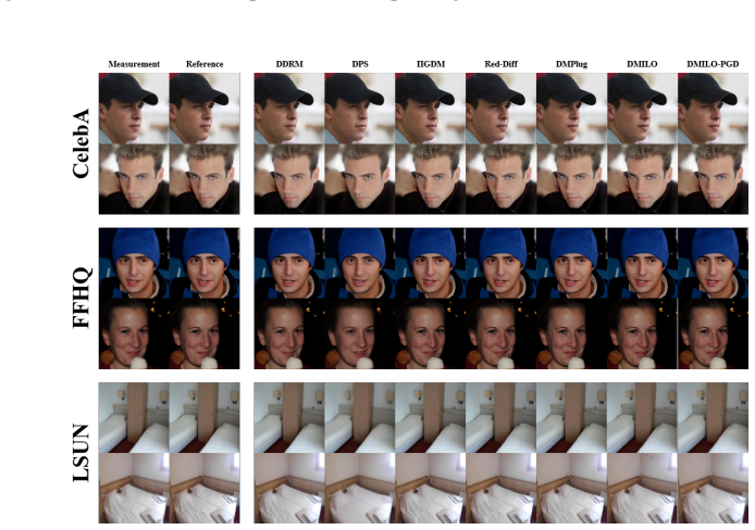
- On nonlinear deblurring, DMILO and DMILO-PGD beat all compared methods on all reported metrics on CelebA and FFHQ, improving PSNR over DMPlug by roughly 2.5 dB.
- The sparse-deviation term consistently improves LPIPS, PSNR, and SSIM in the super-resolution ablation on CelebA.
- Optimizing only the last sampling step (LTS) keeps part of the gain but not all of it, indicating that the multi-step composition contributes to final reconstruction quality.
Reading between the lines
- If the per-step memory claim holds for much longer chains, the same trick could make full-chain latent optimization tractable for high-resolution 3D or video inverse problems, where DMPlug-style methods currently run out of memory.
- The paper's own results show DMILO-PGD degrading on Gaussian deblurring and blind deblurring; a plausible reading is that the naive gradient update on the estimated blur kernel is the weak component, and a kernel parameterization inside a low-dimensional space might restore performance.
- The last-timestep-only experiment suggests a testable initialization rule: choose the initial latent so that $g_N \circ \cdots \circ g_2(z)$ lands near the mode of $g_1$'s input distribution, which could make single-step optimization nearly as good as the full chain.
- Because Theorem 4.4 is stated for global optima over an extended range, the same covering-number argument should transfer to any Lipschitz generative prior with a sparse-deviation term; a direct check would be to run the two-step analysis on a GAN generator and compare sample complexity.
Editorial analysis
A structured set of objections, weighed in public.
Referee Report
Summary. This paper proposes DMILO and DMILO-PGD, two diffusion-model-based inverse problem solvers built on DMPlug. DMILO decomposes the DDIM sampling chain into per-step functions g_i and approximately solves layer-wise objectives (Eqs. (12)-(13)) with Adam, introducing sparse deviations to expand the effective range of the generator. DMILO-PGD alternates a gradient descent step in image space with a DMILO-based projection step. The paper reports memory and runtime reductions relative to the non-checkpointed DMPlug baseline and presents experiments on super-resolution, inpainting, linear and nonlinear deblurring, and blind image deblurring. The theoretical section adapts a result from Daras et al. (2021) to give a measurement-optimality bound for a two-step generator.
Significance. If the central claims held, the paper would provide a practically useful drop-in alternative to DMPlug: per-step optimization reduces the backpropagation graph, wall-clock time, and peak memory relative to the standard DMPlug implementation, and the sparse-deviation mechanism is a reasonable way to relax the generator range. The paper ships code, includes ablations of sparse deviations, and reports memory/time comparisons. However, the theoretical result does not match the implemented algorithm, the memory advantage disappears relative to gradient checkpointing, and the empirical gains are highly task-dependent, with clear failures on Gaussian deblurring and blind image deblurring. These issues make the contribution narrower than the abstract's claims of significant universal gains.
major comments (4)
- [Section 4, Theorem 4.4 and Eq. (18)] The theorem optimizes over x1 ∈ X2 + B_1^n(r), so the sparse deviation is added to the input of g1, and the objective is ∥Ax∗ − A g1(x1)∥2. In the implemented algorithms, Eqs. (12)-(13) and Algorithms 1-2 instead optimize over (x, ν) with g1(x)+ν or g_i(x)+ν, i.e., the deviation is added after the nonlinear DDIM step g_i. These two descriptions coincide only when g1 is affine, but g1 in Eq. (10) is nonlinear. Consequently, the S-REC and covering-number argument over g1(X2 + B_1^n(r)) does not cover the implemented search set {g1(x)+ν : x ∈ X2, ∥ν∥1 ≤ r}, and Theorem 4.4 cannot be invoked as support for the measurement-guided projection in DMILO-PGD. The proof in Appendix A inherits the same mismatch.
- [Section 3.1, Eq. (12)] When A has full row rank with m < n, as in all experiments, for any x one can choose ν so that A(g1(x)+ν)=y exactly, zeroing the quadratic data term in Eq. (12) and leaving only λ∥ν∥1 to enforce data consistency. The paper does not analyze this degeneracy or provide a principled criterion for selecting λ. Without such control, the output-side sparse deviation can make the measurement-matching objective vacuous, which may explain the large performance swings observed for DMILO-PGD in Tables 6-7.
- [Section 5.2, Table 3 and Section 5.4, Tables 6-7] The abstract and contributions claim 'significant performance gains over state-of-the-art methods' and mitigation of suboptimal convergence, but the results are strongly task-dependent. In Table 3 (Gaussian deblurring, ImageNet), DMILO-PGD has FID 164.42 versus 62.67 for DCPS and is also worse than DMPlug; in Tables 6-7 (blind image deblurring), DMILO-PGD degrades dramatically relative to DMILO, for example LPIPS 0.428 versus 0.109 on CelebA with a Gaussian kernel. These are not minor fluctuations but qualitative failures, so the central claim of consistent or even typical superiority over state-of-the-art methods is not supported.
- [Appendix C.4, Table 11] The memory-saving claim is only partially supported. Table 11 shows DMPlug-Ckpt using 3.01 GB, while DMILO and DMILO-PGD use 3.33 and 3.34 GB. Thus, compared with a gradient-checkpointed DMPlug, the proposed methods do not reduce memory. The paper's memory claim should be restricted to the non-checkpointed DMPlug baseline and should explicitly acknowledge the trade-off shown in the same table.
minor comments (5)
- [Appendix B, Algorithm 3] In step 7, 'initailized' is a typo for 'initialized'.
- [Section 3.2, first paragraph] The phrase 'sorely minimize' should be 'solely minimize', and 'without participant of forward operator' should be rephrased as 'without the participation of the forward operator'.
- [Tables 6 and 7, caption] The row labeled 'Ours vs. Best comp.' appears to compare DMILO's performance with the best competitor, not DMILO-PGD's, which is confusing in a table that reports both methods.
- [Section 3.1, Eq. (12)] The text says A(x̂_t0) is replaced by y because the estimated signal is unavailable, but this replacement changes the objective from a comparison with a noisy estimate to a comparison with the noisy observation; the resulting approximation error should be discussed explicitly.
- [Section 5.4, first paragraph] The conjecture that DMILO-PGD's poor BID results are due to the naive gradient update being unsuited for kernel updates is plausible but not directly tested; a brief ablation varying the outer learning rate on the kernel would help.
Circularity Check
No significant circularity: the only theorem is an explicit adaptation of Daras et al. (2021); the empirical claims are benchmark-tested; footnote 3 and the l1-deviation degeneracy are overclaims/correctness risks, not reductions to the paper's inputs.
full rationale
The derivation chain is self-contained rather than circular. Theorem 4.4 is transparently an adaptation of an external result: the paper states 'we adapt the result from (Daras et al., 2021, Theorem 1) to derive the following theorem,' and Appendix A reproduces the standard S-REC chaining (credited to Bora et al., 2017, and Liu & Scarlett, 2020a) with Lemma A.1 (Vempala, 2005). The theorem assumes Lipschitz continuity (Assumption 4.1) and a covering-number bound on the intermediate range (Assumption 4.2), then proves a conditional guarantee relating the measurement optimum to the true optimum; it does not assume its own conclusion. The central empirical claims are benchmark comparisons against independent baselines under fixed hyperparameters; no test-set parameter is fitted and then renamed a prediction, and the 'Ours vs. Best comp.' rows honestly report several losses (e.g., DMILO-PGD FID on Gaussian deblurring). The only self-citation, Liu & Scarlett (2020a) in Appendix A for chaining arguments, is not load-bearing because the same argument is also credited to Bora et al. (2017), an independent source. Two overclaims are flagged as correctness risks rather than circularity. First, footnote 3 asserts that (18) can be regarded as a variant of (12), but (18) adds the sparse deviation to the input of g1 (x1 in X2 + B(r)) while implemented (12) adds it to the output (g1(x)+nu); since g1 in Eq. (10) is nonlinear, the S-REC/covering argument over g1(X2 + B(r)) does not cover the implemented search set. Second, for A in R^(m x n) with m < n and full row rank, nu can be chosen to make A(g1(x)+nu)-y = 0 for any x, so the data term in (12) is trivially satisfiable and lambda*||nu||_1 becomes the effective objective. The paper's own limitations (Sec. 5.4: 'DMILO-PGD shows relatively less effectiveness' in BID; App. C.2: last-timestep-only optimization 'leads to a slight degradation') further show the empirical claims are not manufactured. Overall score 1 corresponds to no significant circularity.
Assumptions & free parameters
free parameters (4)
- lambda (sparse deviation weight) =
0.1
- Adam inner learning rate per task =
0.01 to 0.02
- PGD outer learning rate eta =
0.3 to 8 depending on task
- Inner and outer iteration counts =
200 to 500 inner, 5 to 10 outer
assumptions (6)
- domain assumption Assumption 4.1: g1 is L1-Lipschitz continuous
- domain assumption Assumption 4.2: range of g2 has low intrinsic dimension with covering-number bound log Nδ(X2) ≤ Cg2 k2 log(n/δ)
- standard math Gaussian measurement matrix satisfies S-REC(X-X, γ, δ) with high probability when m is large
- domain assumption The DDIM update gi in Eq. (10) exactly represents each sampling step and its composition G=g1∘...∘gN
- ad hoc to paper Adam approximately solves the layer-wise optimization problems (12)-(13) to near-global optimality
- domain assumption The target signal lies in the extended range g1(X2+B1(r)) for small r = kδ/L1
Cite this review
Pith. "Pith review of Integrating Intermediate Layer Optimization and Projected Gradient Descent for Solving Inverse Problems with Diffusion Models." pith.science (2026). https://pith.science/paper/MWA65GQF
@misc{pith2026250520789,
  author       = {Pith},
  title        = {Pith review of: Integrating Intermediate Layer Optimization and Projected Gradient Descent for Solving Inverse Problems with Diffusion Models},
  year         = {2026},
  howpublished = {\url{https://pith.science/paper/MWA65GQF}},
  note         = {Machine review of arXiv:2505.20789}
}
read the original abstract
Inverse problems (IPs) involve reconstructing signals from noisy observations. Recently, diffusion models (DMs) have emerged as a powerful framework for solving IPs, achieving remarkable reconstruction performance. However, existing DM-based methods frequently encounter issues such as heavy computational demands and suboptimal convergence. In this work, building upon the idea of the recent work DMPlug, we propose two novel methods, DMILO and DMILO-PGD, to address these challenges. Our first method, DMILO, employs intermediate layer optimization (ILO) to alleviate the memory burden inherent in DMPlug. Additionally, by introducing sparse deviations, we expand the range of DMs, enabling the exploration of underlying signals that may lie outside the range of the diffusion model. We further propose DMILO-PGD, which integrates ILO with projected gradient descent (PGD), thereby reducing the risk of suboptimal convergence. We provide an intuitive theoretical analysis of our approaches under appropriate conditions and validate their superiority through extensive experiments on diverse image datasets, encompassing both linear and nonlinear IPs. Our results demonstrate significant performance gains over state-of-the-art methods, highlighting the effectiveness of DMILO and DMILO-PGD in addressing common challenges in DM-based IP solvers.
Figures


Figures from the paper (7 more)




Reference graph
Works this paper leans on
-
[1]
(20) Based on Lemma A.1 and Assumptions 4.1 and 4.2, we present the proof of Theorem 4.4 as follows
that P (1 − ϵ)∥x∥2 2 ≤ ∥Ax∥2 2 ≤ (1 + ϵ)∥x∥2 2 ≥ 1 − 2e−ϵ2(1−ϵ)m/4. (20) Based on Lemma A.1 and Assumptions 4.1 and 4.2, we present the proof of Theorem 4.4 as follows. A.1. Proof of Theorem 4.4 From Assumption 4.2, we have log N δ L1 (X2) ≤ Cg2 k2 log L1n δ . (21) Additionally, using Maurey’s Empirical Method (see (Daras et al., 2021, Theorem 2)), we can...
work page 2021
-
[3]
Progressive growing of GANs for improved quality, stability, and variation
Karras, T., Aila, T., Laine, S., and Lehtinen, J. Progressive growing of GANs for improved quality, stability, and variation. https://arxiv.org/abs/1710.10196,
-
[4]
w/” denotes methods that utilize sparse deviations, and “w/o
This completes the proof. B. Algorithms for BID Following the kernel estimation method proposed in DMPlug (Wang et al., 2024), we incorporate it into our framework and present the complete algorithms for our methods DMILO and DMILO-PGD for blind image deblurring tasks in Algorithms 3 and 4, respectively. 14 Integrating Intermediate Layer Optimization and ...
work page 2024
-
[6]
Consistency model is an effective posterior sample approximation for diffusion inverse solvers
Xu, T., Zhu, Z., Li, J., He, D., Wang, Y ., Sun, M., Li, L., Qin, H., Wang, Y ., Liu, J., and Zhang, Y .-Q. Consistency model is an effective posterior sample approximation for diffusion inverse solvers. https://arxiv.org/abs/2403.12063,
-
[8]
Zhang, J., Liu, Z., Yan, L., Li, G., and Gu, Y . Improving diffusion-based inverse algorithms under few-step con- straint via learnable linear extrapolation. arXiv preprint arXiv:2503.10103, 2025b. Zhang, K., Li, Y ., Zuo, W., Zhang, L., Van Gool, L., and Timofte, R. Plug-and-play image restoration with deep denoiser prior. IEEE Transactions on Pattern An...
-
[9]
13 Integrating Intermediate Layer Optimization and Projected Gradient Descent for Solving Inverse Problems with Diffusion Models A. Proof of Theorem 4.4 First, we present the following basic concentration inequality for the Gaussian measurement matrix. Lemma A.1. (Vempala, 2005, Lemma 1.3) Suppose that A ∈ Rm×n has i.i.d. N (0, 1/m) entries. For fixed x ∈...
work page 2005
-
[11]
≤ k2 log(3n). (23) Moreover, since g1 is L1-Lipschitz continuous, if M is a (δ/L1)-net of X2 + Bn 1 (r), we have that g1(M ) is a δ-net of g1 X2 + Bn 1 (r) . Therefore, letting X = g1 X2 + Bn 1 (r) , we have log Nδ(X ) ≤ Cg2 k2 log L1n δ + k2 log(3n). (24) Then, based on Lemma A.1 and the well-established chaining arguments in (Bora et al., 2017; Liu & Sc...
work page 2017
-
[2015]
Sohoni, N. S., Aberger, C. R., Leszczynski, M., Zhang, J., and R ´e, C. Low-memory neural network training: A technical report. https://arxiv.org/abs/1904.10631,
arXiv 1904
Show all 12 references
-
[2017]
LSUN: Construction of a large-scale image dataset using deep learning with humans in the loop
Yu, F., Zhang, Y ., Song, S., Seff, A., and Xiao, J. LSUN: Construction of a large-scale image dataset using deep learning with humans in the loop. https://arxiv.org/abs/1506.03365,
-
[2023]
Feng, B. T. and Bouman, K. L. Efficient Bayesian com- putational imaging with a surrogate score-based prior. https://arxiv.org/abs/2309.01949,
-
[2024]
DPM- Solver: A fast ODE solver for diffusion probabilistic model sampling in around 10 steps
Lu, C., Zhou, Y ., Bao, F., Chen, J., Li, C., and Zhu, J. DPM- Solver: A fast ODE solver for diffusion probabilistic model sampling in around 10 steps. In NeurIPS, 2022a. 11 Integrating Intermediate Layer Optimization and Projected Gradient Descent for Solving Inverse Problems...
-
[2025]
Chen, S., Chewi, S., Li, J., Li, Y ., Salim, A., and Zhang, A. R. Sampling is as easy as learning the score: The- ory for diffusion models with minimal data assumptions. https://arxiv.org/abs/2209.11215,
Reviewed August 7, 2026 · model on record in the stance chip above.
Discussion (0). Continue with ORCID to comment.