REVIEW 2 major objections 5 minor 51 references
Fisher information from quantum many-particle arrival time measurements
T0 review · 2 major / 5 minor · reviewed 2026-08-07 · deepseek-v4-flash
Pith's one-line read The paper derives exact Fisher information for momentum estimation from arrival times of Bosonic beams, showing that sparse-beam arrival times carry nonzero information about $p_0$ even when the beam's position distribution is flat.
desk verdict Solid analytical contribution on Fisher information from arrival times; the sparse-beam limits are the real news and hold, but the dense-beam limit proof needs a fix and the infinite-horizon caveat matters. read the letter →
The pith
A machine-rendered reading of the paper's core claim, the machinery that carries it, and where it could break.
The reading
What carries the argument
The load-bearing object is the absorptive detection model: a Lindblad master equation on the Bosonic Fock space whose jump operator $a(\phi)$ annihilates a particle in the absorbing state $\phi$ (eq. (6)). Unravelling gives the arrival-time densities $p_n(t)=F_n(\Omega(t_n))\prod_{i=1}^n \omega(t_i)$, where $\omega(t)=\langle N\rangle\gamma\,|\langle\phi|\chi_t\rangle|^2$ is the detection intensity, $\Omega$ its integral, and $F$ is $(1-\Omega/N)^N$ for Fock states, $e^{-\Omega}$ for coherent states, and $(1+\Omega)^{-1}$ for quasi-free states. In the point-detector limit the intensity is determined by a Volterra integral equation whose solution splits into a stationary transmission amplitude $T_p$ and a transient term; in the uniform-beam limit the intensity becomes $ar_0|T_{p_0}+R_{p_0}(t)|^2$. The general Fisher-information formula (42), together with the large-time asymptotics of this intensity, yields the sparse-beam limits (45)--(46).
What would settle it
Measure arrival times of a free one-dimensional Bose beam with a point absorber at two densities and for both coherent and thermal (geometric-number) states; estimate $p_0$ by maximum likelihood from the first $n$ arrival times and check that the inverse estimator variance grows as $n$ for coherent states and saturates as $n/(n+2)$ for thermal states, since the paper's predictions differ by exactly the factor $n+2$.
Extended reading notes
Core claim
The central discovery is that the momentum $p_0$ of a beam particle is identifiable from arrival times even though the spatial density of the beam contains no information about it: in the delta-detector and uniform-beam limits with vanishing particle density $r_0\to 0$, the Fisher information from the first $n$ arrival times is nonzero and has the simple form $I_n(p_0)=n\,I_\infty(p_0)$ for coherent states and $I_n(p_0)=\frac{n}{n+2}\,I_\infty(p_0)$ for quasi-free (thermal) states, where $I_\infty(p_0)=\frac{a^2 m^2}{p_0^2(p_0+am/2)^2}$ with $a$ the detection strength and $m$ the particle mass. The paper derives this by first obtaining a general formula for the Fisher information of the arrival-time model, then taking the sparse-beam limit using a dominated-convergence argument; the limiting value coincides with the Fisher information of a hypothetical time-stationary detection model. It also proves that in the opposite dense-beam limit $r_0\to\infty$ the information vanishes, and that in the finite-particle case the information in $n$ detections has a maximum rather than growing monotonically.
Load-bearing premise
The result assumes an unbounded observation window: in the sparse-beam limit the detections happen at arbitrarily late times, so the stated Fisher information corresponds to waiting infinitely long, and any finite-time experiment sees the probability of observing $n$ arrivals vanish.
Editorial extensions
If this is right
- Momentum estimation from temporal data is possible in a regime where position measurements give nothing: the beam's spatial distribution is flat and parameter-free.
- In the beam limit the total probability of observing $n$ arrivals equals 1 for every $n$, so the Fisher information grows with $n$; in any finite-particle beam it instead peaks at an optimal number of detections.
- For sparse beams the scaling differs sharply between state types: each additional arrival adds a constant amount of information for coherent states, while for quasi-free states the information saturates at $I_\infty(p_0)$.
- Increasing the particle density $r_0$ towards infinity drives the Fisher information to zero, so sparse beams are information-optimal within this model.
Reading between the lines
- The nonzero sparse-beam limit is an infinite-time statement: in a finite observation window the probability of collecting $n$ arrivals vanishes as $r_0\to 0$, so achieving the predicted information requires waiting times that diverge as the beam is diluted.
- The ratio $I_n(\text{coherent})/I_n(\text{quasi-free})=n+2$ gives a parameter-free signature of the particle-number statistics (Poisson vs geometric) that could be tested purely from temporal data.
- The same Fisher-information formula applies to any single-particle parameter, so the framework extends to simultaneous estimation of momentum, mass, and detection strength, where correlations between arrival times would matter.
- The predicted transient-vs-stationary structure of the intensity, with its $O(t^{-3/2})$ tail and $p_0$-dependent constant, is directly testable by histogramming first-arrival times of a dilute beam.
Editorial analysis
A structured set of objections, weighed in public.
Referee Report
Summary. The paper constructs a many-particle arrival-time detection model based on a Fock-space absorption master equation, derives the joint arrival-time distributions for Fock, coherent, and quasi-free source states, and then analyzes two idealizing limits: a point (Dirac-delta) detector and a spatially uniform infinite-particle beam. For the beam, the paper derives a tractable formula for the classical Fisher information of the single-particle momentum parameter (Eq. (42)) and studies its dependence on the particle density. The central results are Eqs. (45)-(46): in the sparse-beam limit r0→0, the Fisher information from the first n arrival times tends to n I∞(p0) for coherent states and to n/(n+2) I∞(p0) for quasi-free states, where I∞(p0)=a^2 m^2/[p0^2(p0+am/2)^2]. This limit coincides with the Fisher information of a hypothetical time-stationary detection model, as shown rigorously in Appendix D. The authors emphasize that the spatial particle distribution in the beam contains no information about p0, so the arrival-time data are the only carrier of momentum information.
Significance. If the results are correct, this is a valuable contribution at the interface of quantum arrival-time theory and quantum statistical inference. The paper provides explicit, parameter-free limiting formulas for the Fisher information, and it demonstrates a conceptually striking effect: temporal detection data can encode single-particle parameters even when the spatial statistics are completely insensitive to them. The appendices contain substantial original analysis: Appendix B proves convergence to the delta-detector Volterra equation, Appendix D derives the general Fisher-information formula and the sparse/dense beam limits via dominated convergence. The paper is refreshingly honest in acknowledging some idealizations, such as the need to wait infinitely long in the sparse-beam limit. The main caveat is that the identifiability statement must be understood as an infinite-horizon property, not a finite-time estimation prescription; this is acknowledged in Section IV.C but underemphasized in the abstract. The mathematical core appears sound, though one technical assumption (positivity of the beam intensity) is stated but not verified in the proof of the sparse-beam limit.
major comments (2)
- [Abstract and §IV.C] The nonzero limits (45)–(46) describe the joint density of the first n arrival times on [0,∞)^n. For a coherent beam the full finite-horizon data are a Poisson process with intensity r0 g(t); for fixed T the Fisher information of the parameter p0 is r0 ∫_0^T g(t) (∂_p log g(t))² dt, which tends to zero as r0→0. Thus the statement that the momentum is identifiable in the sparse-beam limit is only an infinite-horizon statement: the information per detected particle survives, but the expected time to the n-th detection diverges as n/(r0 g∞). The paper acknowledges this in §IV.C ('we need to wait infinitely long to get detections'), but the abstract and conclusion phrase the claim as if it were a finite-time estimation property. Please qualify the identifiability claim explicitly.
- [Appendix D.b] The dominated convergence proof of (45)–(46) requires a uniform (in r0) integrable bound on |Fn(u)u^{n-1}S_{n,r0}(u)|. The bound is obtained from a constant A bounding |Φ(t)|, |~Φ(t)|, and |φ(t)| on [0,∞). While Φ and ~Φ are bounded because they are continuous with finite limits, the boundedness of φ(t)=˙g(t)/g(t) requires g(t) to be strictly positive for all t. The manuscript only states the assumption ω(t)>0 at the start of Appendix D; it is not verified for the explicit beam intensity (39). If g had a zero, φ would be unbounded and the stated dominated convergence argument would fail. Please supply a proof of positivity of (39), or state it as a necessary assumption and adapt the proof.
minor comments (5)
- [Appendix D, first paragraph] The text says 'In(p) := E[Vp]'; since Vp is the score, this should read E[Vp²].
- [§II.D.3] The intermediate derivation for the quasi-free state contains garbled factors ('n! Qn...', 'n/q') and should be corrected; the final formula is correct.
- [§II.F] The phrase 'one the other hand' should be 'on the other hand'.
- [Eq. (42)] The text indicates that the second and third terms appear only for n≥2 and the fourth only for n≥3, but the displayed formula does not show this; adding a parenthetical condition in the equation would improve clarity.
- [§III.A] The symbol f(t) is used in the limiting equation before its definition in the surrounding text; a brief definition of f(t) immediately after Eq. (23) would help.
Circularity Check
No load-bearing circularity: sparse-beam Fisher-information limits (45)-(46) are derived by dominated convergence from the absorption model, not imposed by definition or self-citation.
full rationale
The central claims are derived rather than assumed. Section III derives the delta-detector intensity from the Volterra equation (23), whose kernel follows from the free propagator and the delta-limit (22); the beam limit (39) uses the explicit beam definition (30)-(31). The Fisher-information formula (42) is obtained in Appendix D by direct score-function algebra using the Cauchy repeated-integration formula; no fitted constant enters. The sparse-beam limits (45)-(46) are proved in Appendix D.b by dominated convergence, after bounding an r0-independent dominating function, and the constants C(n)=n (coherent) and C(n)=n/(n+2) (quasi-free) are evaluated exactly. The 'coincidence' with the time-stationary model is itself a proven equality: both sides equal C(n)(g_dot_infty/g_infty)^2, and I_infinity(p0) is defined through (36)-(37), not fitted to the Fisher-information result. Self-citations ([4],[5],[25]) are background context: [5] is explicitly distinguished from the present static beam definition in Section III.B, and the master equation comes from external references [36,37]. The only caveat is interpretive: in the sparse-beam limit the nth arrival time diverges as 1/r0, so the finite-time Fisher information vanishes; Section IV.C states this ('we need to wait infinitely long to get detections'). That is an idealization and limitation, not circular reasoning. Accordingly, the score reflects only minor background self-citation; no step reduces to its own input.
Assumptions & free parameters
assumptions (6)
- domain assumption The many-particle detection process is governed by the Lindblad master equation (6) with L = a(phi), taken from [36,37].
- domain assumption The delta detector limit is defined by sqrt(gamma_epsilon) phi_epsilon -> sqrt(a) delta(x), and the intensity is obtained as the limit of solutions of the Volterra equation (23).
- domain assumption The infinite uniform beam is defined by the Fock-space limit (30)-(31) with constant spatial density r0 and definite momentum p0; arrival time distributions are taken as the limit of finite-mean-N distributions.
- domain assumption The source wavefunction's Fourier transform is integrable, so that the free evolved wavefunction is continuous and the delta-detector convergence applies.
- domain assumption The intensity omega(t) is strictly positive for all t > 0, so the substitution u = Omega(t) in Appendix D is invertible.
- standard math Standard Volterra integral equation theory and Laplace transform methods, including the convergence argument from [44], are valid for Eq. (23) and its finite-regularization approximations.
Cite this review
Pith. "Pith review of Fisher information from quantum many-particle arrival time measurements." pith.science (2026). https://pith.science/paper/5JPNJXD2
@misc{pith2026250521214,
  author       = {Pith},
  title        = {Pith review of: Fisher information from quantum many-particle arrival time measurements},
  year         = {2026},
  howpublished = {\url{https://pith.science/paper/5JPNJXD2}},
  note         = {Machine review of arXiv:2505.21214}
}
abstract
We formulate a quantum arrival time measurement process for a Bosonic many-particle system, with the aim of extracting statistical information on single-particle properties. The arrival time is based on a dynamical multi-particle absorption model in the Fock space, and we consider systems in coherent and incoherent mixtures of $N$-particle states. We find the resulting probability distributions for arrival time sequences, which we consider as parametric models for the statistical inference of single-particle parameters, and derive a tractable expression for the associated (classical) Fisher information. Subsequently focusing on the concrete case of the momentum parameter of a 1D particle, we consider the idealized limits of a point (Dirac delta) detector and an infinite particle system forming a spatially uniform ``beam''. We observe that even though no information remains in the spatial distribution, the single-particle momentum is indeed identifiable from the arrival time data, even in the limit of ``sparse beams'' of vanishing particle density, where we obtain simple analytical form for the Fisher information, which, interestingly, coincides with the one obtained from a hypothetical time-stationary detection model. Our results contribute to the fundamental understanding of temporal measurement data arising from quantum systems consisting of freely evolving particles.
Figures


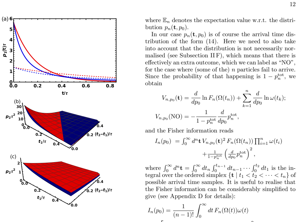
Figures from the paper (4 more)


Reference graph
Works this paper leans on
-
[1]
We now evaluate the density pn(t), for each fixed number n of arrivals
Fock states Consider the Fock state ρ = |χ⊗N ⟩⟨χ⊗N |, where N is fixed, so that the state lies in the N -particle sector of the Fock space. We now evaluate the density pn(t), for each fixed number n of arrivals. Noting first that by the definition of Jt, we get Jt|ψ⊗N ⟩ = a(ϕ)|(Utψ)⊗N ⟩ = √ N ⟨ϕ|Utψ⟩|(Utψ)⊗N −1⟩ for any ψ and t. Consider now two detection...
-
[2]
Coherent states We now consider the coherent states ρ = |Ψ⟩⟨Ψ|, Ψ = ∞M N =0 ⟨N ⟩ N 2 e−⟨N ⟩/2 √ N ! |χ⊗N ⟩ ∈H. (11) These are quantum superpositions of Fock states, in such a way that the particle number distribution is Poisson with mean ⟨N ⟩. Analogous to the Fock state case, we define ω(t) = ⟨N ⟩γ|⟨ϕ|χt⟩|2, Ω(t) = Z t 0 ω(t′)dt′, (12) noting that this i...
-
[3]
Quasi-free states Finally, we study specific classical mixtures of Fock states, generated via a simple Bernoulli trial (coin toss) sequence: at each trial a particle is created with prob- ability β, and the trials are repeated until the first failure. (One can think of an “oven” emitting parti- cles, in which case β would be related to temperature.) Hence...
-
[4]
Tunneling Times with Covariant Measurements
J. Kiukas, A. Ruschhaupt and R. F. Werner, “Tunneling Times with Covariant Measurements”, Found. Phys. 39, 829 (2009)
work page 2009
-
[5]
Arrival Time in Quantum Mechanics
J. G. Muga, C. R. Leavens, “Arrival Time in Quantum Mechanics”, Phys. Rep. 338, 353 (2000)
work page 2000
-
[6]
J. G. Muga, R. Sala Mayato and I. L. Egusquiza (eds.) 24 Time in quantum mechanics (Lect. Notes Phys. m72, Springer, Berlin) (2002)
work page 2002
-
[7]
J. G. Muga, A. Ruschhaupt and A. del Campo (eds.) Time in quantum mechanics – Vol.2(Lect. Notes Phys. 789, Springer) (2009)
work page 2009
-
[8]
Arrival Time in Quantum Mechanics
J. Kijowski, “Arrival Time in Quantum Mechanics”, Acta Phys. Pol A 143, s123 (2023)
work page 2023
Show all 51 references
-
[9]
Full count- ing statistics of stationary particle beams
J. Kiukas, A. Ruschhaupt and R. F. Werner, “Full count- ing statistics of stationary particle beams”, J. Math. Phys. 54, 042109 (2013)
2013
-
[10]
Quantum Measurement of Time
L. Maccone and K. Sacha, “Quantum Measurement of Time”, Phys. Rev. Lett. 124, 110402 (2020)
2020
-
[11]
When does a particle arrive?
S. Roncallo, K. Sacha and L. Maccone, “When does a particle arrive?”, Quantum 7, 968 (2023)
2023
-
[12]
Pauli: in Encyclopedia of Physics, ed
W. Pauli: in Encyclopedia of Physics, ed. by S. Flugge (Springer, Berlin), Vol. V/1, p. 60 305 (1958)
1958
-
[13]
Evolution with- out evolution: Dynamics described by stationary observ- ables
D. N. Page and William K. Wootters, “Evolution with- out evolution: Dynamics described by stationary observ- ables”, Phys. Rev. D 27, 2885–2892 (1983)
1983
-
[14]
Quantum Time
V. Giovannetti, S. Lloyd and L. Maccone, “Quantum Time”, Phys. Rev. D 92, 045033 (2015)
2015
-
[15]
Evolution without evolu- tion, and without ambiguities
C. Marletto and V. Vedral, “Evolution without evolu- tion, and without ambiguities”, Phys. Rev. D 95, 043510 (2017)
2017
-
[16]
Screen observables in relativistic and non- relativistic quantum mechanics
R. Werner, “Screen observables in relativistic and non- relativistic quantum mechanics”, J. Math. Phys. 27, 793 (1986)
1986
-
[17]
Time in the Quantum The- ory and the Uncertainty Relation for Time and Energy
Y. Aharonov and D. Bohm, “Time in the Quantum The- ory and the Uncertainty Relation for Time and Energy”, Phys. Rev. 122, 1649 (1961)
1961
-
[18]
On the Time Operator in Quantum Me- chanics and the Heisenberg Uncertainty Relation for En- ergy and Time
J. Kijowski, “On the Time Operator in Quantum Me- chanics and the Heisenberg Uncertainty Relation for En- ergy and Time”, Rep. Math. Phys. 6, 361 (1974)
1974
-
[19]
‘Standard’ quantum mechanical approach to times of arrival
I. L. Egusquiza, J. G. Muga and A. D. Baute, “‘Standard’ quantum mechanical approach to times of arrival”, in [2]
-
[20]
De- tector models for the quantum time of arrival
A. Ruschhaupt, J. G. Muga and G. C. Hegerfeldt, “De- tector models for the quantum time of arrival”, in [3]
-
[21]
Inequalities expressing the Pauli principle for generalized observables
R. F. Werner, “Inequalities expressing the Pauli principle for generalized observables”, in Mathematical methods in statistical mechanics (Leuven Univ. Press), pp. 179 -196 (1989)
1989
-
[22]
Quantum times of arrival for multiparticle states
A.D. Baute, I.L. Egusquiza, J.G. Muga, “Quantum times of arrival for multiparticle states”, Phys. Rev. A 65, 032114 (2002)
2002
-
[23]
Measurement-based approach to quantum arrival times
J.A. Damborenea, I.L. Egusquiza, G.C. Hegerfeldt, J.G. Muga, “Measurement-based approach to quantum arrival times”, Phys. Rev. A 66, 052104 (2002)
2002
-
[24]
Perfect detec- tion of ultra-cold atoms by laser-induced ionization
A. Ruschhaupt, B. Navarro, J. G. Muga, “Perfect detec- tion of ultra-cold atoms by laser-induced ionization”, J. Phys. B: At. Mol. Opt. Phys. 37, L313 (2004)
2004
-
[25]
The Time of Arrival in Quantum Mechan- ics
G.R. Allcock, “The Time of Arrival in Quantum Mechan- ics”, Ann. Phys. (N.Y.) 53, 253 (1969); 53, 286 (1969); 53, 311 (1969)
1969
-
[26]
Arrival Time Observables in Quantum Me- chanics
R. Werner, “Arrival Time Observables in Quantum Me- chanics”, Ann. Inst. Henri Poincar´ e47, 429 (1987)
1987
-
[27]
Exact and approximate com- plex potentials for modelling time observables
A. Ruschhaupt, J.A. Damborenea, B. Navarro, J.G. Muga, G.C. Hegerfeldt, “Exact and approximate com- plex potentials for modelling time observables”, Euro- phys. Lett. 67, 1 (2004)
2004
-
[28]
Carmichael, An Open Systems Approach to Quantum Optics (Springer, Berlin, 1993)
H. Carmichael, An Open Systems Approach to Quantum Optics (Springer, Berlin, 1993)
1993
-
[29]
Exact energy–time uncertainty relation for ar- rival time by absorption
J. Kiukas, A. Ruschhaupt, P. O. Schmidt and R. F. Werner, “Exact energy–time uncertainty relation for ar- rival time by absorption”, J. Phys. A: Math. Theor. 45, 185301 (2012)
2012
-
[30]
Hegerfeldt, T.S
G.C. Hegerfeldt, T.S. Wilser, in Classical and Quan- tum Systems. Proceedings of the Second International Wigner Symposium, July 1991, ed. by H.D. Doebner, W. Scherer, F. Schroeck, (World Scientific, Singapore, 1992), p. 104; G.C. Hegerfeldt, Phys. Rev. A 47, 449 (1993); G.C. ...
1993
-
[31]
Dalibard, Y
J. Dalibard, Y. Castin, K. Mølmer, Phys. Rev. Lett. 68, 580 (1992)
1992
-
[32]
Continuous matrix prod- uct states for quantum fields
F. Verstraete and J. I. Cirac, “Continuous matrix prod- uct states for quantum fields”, Phys. Rev. Lett. 104 190405 (2010)
2010
-
[33]
E. P. Davies, Quantum Theory of Open Systems, Aca- demic Press, London 1976
1976
-
[34]
Measurement theory and stochastic dif- ferential equations in quantum mechanics
A. Barchielli, “Measurement theory and stochastic dif- ferential equations in quantum mechanics”, Phys. Rev. A. 34 1642 (1986)
1986
-
[35]
Finitely cor- related states on quantum spin chains
M. Fannes, B. Nachtergaele, R.F. Werner, “Finitely cor- related states on quantum spin chains”, Commun. Math. Phys. 144 443 (1992)
1992
-
[36]
General Theory and Applications to Unstable Particles
R. Alicki, “General Theory and Applications to Unstable Particles”, Lect. Notes Phys. 717, 1-46, Springer, Berlin (2007)
2007
-
[37]
Quantum collision models: Open system dynamics from repeated interactions
F. Ciccarello, S. Lorenzo, V. Giovannetti, G. M. Palma, “Quantum collision models: Open system dynamics from repeated interactions”, Physics Reports 954 1-70 (2022)
2022
-
[38]
Lindblad, Commun
G. Lindblad, Commun. Math. Phys. 48, 119-130 (1976)
1976
-
[39]
Gorini, A
V. Gorini, A. Kossakowski, E. C. G. Sudarshan, Math. Phys. 17, 821 (1976)
1976
-
[40]
An Introduction to the Theory of Point Processes
D. Daley and D. Vere-Jones, “An Introduction to the Theory of Point Processes” (2 vols.) (Springer, 1988)
1988
-
[41]
Dynamical phase transition for a quantum particle source
M. Butz and H. Spohn, “Dynamical phase transition for a quantum particle source”, Ann. Henri Poincar´ e10, 1223– 1249 (2010)
2010
-
[42]
Detection and ’emission’ pro- cesses of quantum particles in a ’chaotic state’
C. B´ enard and O. Macchi, “Detection and ’emission’ pro- cesses of quantum particles in a ’chaotic state’”, J. Math. Phys. 14, 155 - 167 (1973)
1973
-
[43]
Operator Algebras and Quantum Statistical Mechanics II
O. Bratteli and D. W. Robinson, “Operator Algebras and Quantum Statistical Mechanics II” (Springer, Berlin, 1997)
1997
-
[44]
On Linear Volterra Integral Equations of Con- volution Type
J. S. Lew, “On Linear Volterra Integral Equations of Con- volution Type”, Proceedings of the American Mathemat- ical Society. 35, 450-456 (1972)
1972
-
[45]
Random point processes in time and space
D. L. Snyder and M. I. Miller, “Random point processes in time and space” (Springer New York, 1991)
1991
-
[46]
Gregoire, “Negative binomial distributions for point processes, Stochastic processes and their applications 16 179 (1983)
G. Gregoire, “Negative binomial distributions for point processes, Stochastic processes and their applications 16 179 (1983)
1983
-
[47]
Handbook of Mathe- matical Functions
M. Abramowitz, I. A. Stegun, “Handbook of Mathe- matical Functions” (Dover Publications, Inc., New York, 1965)
1965
-
[49]
The Laplace transform
R. E. Bellman, R. S. Roth, “The Laplace transform”, World Scientific, Singapore, 1984
1984
-
[50]
Statistical Inference
P. H. Garthwaite, I. T. Jolliffe, B. Jones, “Statistical Inference”, 2nd Edition (Oxford University Press, New York, 2006)
2006
-
[51]
Quantum estimation for quantum technol- ogy
M. A. Paris, “Quantum estimation for quantum technol- ogy”, Int. J. Quant. Inf. 7 125 (2009)
2009
-
[100]
Dirac delta
For this particle number, the coherent and Fock results are essentially indistinguishable; it is well known that the Fock state and the coherent state converge to each other for large particle number and this can be seen also here. Different widths of the absorbing state are c...
2000
Reviewed August 7, 2026 · model on record in the stance chip above.
Discussion (0). Sign in to comment.