REVIEW 2 major objections 7 minor 4 cited by
The James Webb Space Telescope NIRSpec-PRISM Transmission Spectrum of the Super-Puff, Kepler-51d
T0 review · 2 major / 7 minor · reviewed 2026-08-07 · deepseek-v4-flash
Pith's one-line read JWST transmission spectroscopy of super-puff Kepler-51d shows a sloped, featureless spectrum best explained by a low-metallicity H/He atmosphere with high-altitude submicron hazes, ruling out a massive ring and starspots as the source of…
desk verdict First JWST spectrum of a super-puff; the slope is real and consistent across pipelines, the haze interpretation is the best available, but the limb-darkening robustness check is missing and the ring alternative is not fully closed. read the letter →
The pith
A machine-rendered reading of the paper's core claim, the machinery that carries it, and where it could break.
The reading
What carries the argument
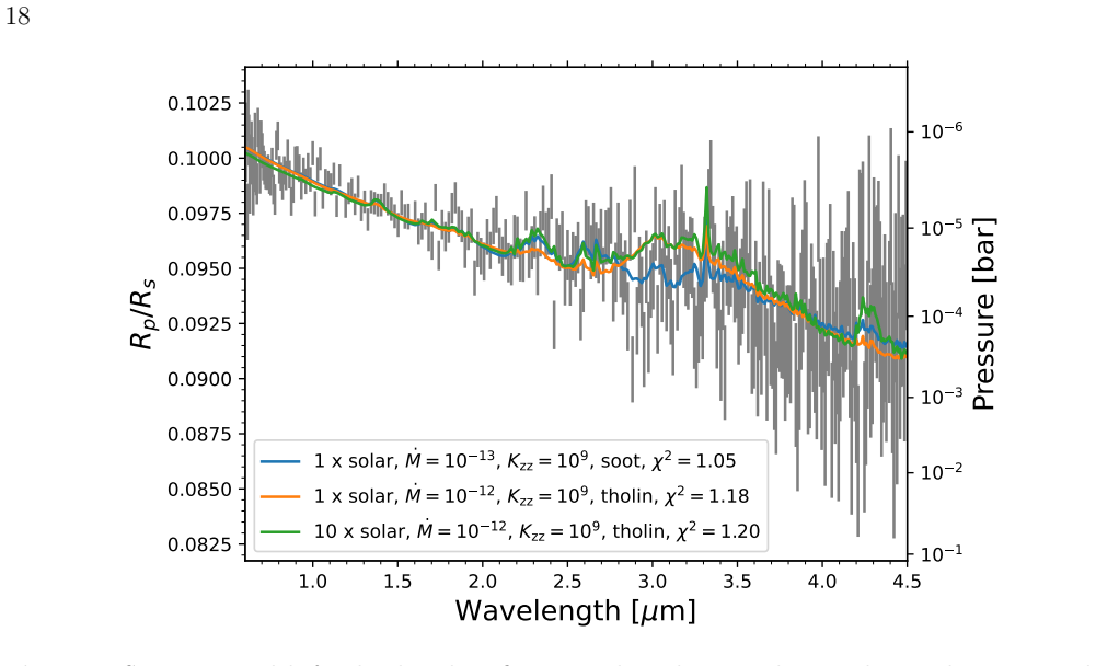
The load-bearing object is the wavelength-dependent transit-depth slope, interpreted as the altitude at which the atmosphere becomes optically thick at each wavelength. Submicron haze particles scatter more strongly at short wavelengths, pushing the effective transit radius outward toward the blue and producing a steep, featureless slope; reproducing its steepness requires a low-metallicity, large-scale-height atmosphere, a moderate haze production rate, and strong vertical mixing. The paper supports this with three independent lines: Bayesian atmospheric retrievals on an isothermal H/He atmosphere, a physically motivated forward model of haze microphysics and transport, and a ring-retrieval model used to estimate the alternative ring's lifetime under Poynting-Robertson drag.
What would settle it
Re-fit the same NIRSpec light curves with limb-darkening coefficients fixed to stellar-model values (or with a physically motivated prior), include the 4.5–5.3 micron channels, and check whether the 0.6–4.5 micron slope survives; if the slope flattens or a blue turnover appears, the high-altitude haze conclusion would not stand. A second independent transit observation at higher signal-to-noise, or detection of ring-induced oblateness or transit-depth changes over years, would also discriminate haze from a transient ring.
Extended reading notes
Core claim
On its own terms, the paper discovers that Kepler-51d's 0.6–5.3 μm transmission spectrum is a smooth slope spanning about 0.75 Earth radii, with no molecular absorption features robustly detected. The authors argue this slope is best explained by a low-metallicity H/He envelope topped by a thick high-altitude haze of submicron particles that becomes optically thick at 1–10 microbars and spans roughly 1–100 microbars. They further claim that stellar spots cannot produce the slope on their own, that a massive opaque ring is ruled out, and that an optically thin tilted ring, although able to fit the data, has a lifetime of only about 0.1 million years under Poynting-Robertson drag, far shorter than the 500-million-year system age. The methane hint at 2.2 sigma is treated as tentative and potentially an upwelling artifact.
Load-bearing premise
The haze conclusion rests on treating the measured 0.6–4.5 micron slope as genuine planetary extinction while limb-darkening parameters are fit freely and the noisy reddest channels are ignored; if that slope is partly an artifact of those choices, the haze interpretation weakens.
Editorial extensions
If this is right
- Kepler-51d's inflated radius requires both a massive H/He envelope (roughly 30% of its mass) and an optically thick high-altitude haze; the haze alone cannot explain the radius.
- The 1–100 microbar haze layer implies that transmission spectra of such planets probe pressures far above the 1–100 mbar region usually assumed, so recovered radii correspond to very low pressures.
- Massive opaque circumplanetary rings are ruled out as an explanation for super-puff radii, leaving only short-lived optically thin rings as a viable ring scenario.
- The result supports a population picture in which cool Neptunes and sub-Neptunes around 300–500 K are prime haze producers, consistent with earlier HST-based trends.
- Unocculted starspots cannot reproduce the >2 micron slope, so the spectrum is a genuine atmospheric signal, and the spot crossing gives a spot temperature roughly 200–300 K cooler than the photosphere, hotter than typical sunspot umbras.
Reading between the lines
- If the haze interpretation holds, Kepler-51b and Kepler-51c should show similarly sloped JWST transmission spectra; observing them would test whether all three super-puffs share one haze mechanism.
- A re-analysis that fits limb darkening with stellar-model priors and includes wavelengths beyond 4.5 microns could either confirm or weaken the slope, since the paper does not quantify how much the derived haze parameters change under alternative limb-darkening treatments.
- The short ring lifetime implies that any genuine ring detection would indicate very recent dynamical events, so repeated transit observations over years could distinguish a transient ring from a stable haze layer.
- The retrieved particle sizes are slightly larger than the forward-model sizes (0.15–0.35 microns versus about 0.1 microns), so higher signal-to-noise data or broader wavelength coverage could discriminate particle composition and shape models, including fluffy aggregates.
Editorial analysis
A structured set of objections, weighed in public.
Referee Report
Summary. The paper presents a JWST NIRSpec-PRISM 0.6–5.3 µm transmission spectrum of the super-puff Kepler-51d, obtained from a single transit. The authors reduce the data with three independent pipelines (Eureka!, ExoTiC-JEDI, and chromatic/starry) and find consistent, near-featureless spectra with a strong slope in transit depth across 0.6–4.5 µm, corresponding to a planet radius change of about 0.75 R⊕. They model the spectrum with two retrieval codes (ExoTR and PLATON) and with a grid of microphysical forward haze models, concluding that the slope is best explained by high-altitude, submicron hazes in a low-metallicity H/He atmosphere at pressures of 1–100 µbar. They also fit an optically thin tilted ring model, which reproduces the spectrum equally well (reduced χ² = 0.95), but argue the ring is short-lived (~0.1 Myr) from Poynting-Robertson drag. The paper additionally analyzes a starspot crossing event and out-of-transit stellar spectra to rule out stellar contamination as the source of the slope.
Significance. If the haze interpretation holds, this is the first JWST transmission spectrum of a super-puff with a strongly sloped, featureless continuum, providing direct evidence for high-altitude aerosol layers in a cool (T_eq ~350 K) low-gravity planet. The paper has notable strengths: three independent reductions and fitting routines agree, the data and best-fit tables are released in machine-readable form, the forward microphysical models provide an independent physical check on the retrievals, and the analysis explicitly tests alternative explanations (ring, starspots). The result would meaningfully constrain haze formation and transport in a previously unexplored temperature regime. However, the central claim rests on the assumption that the spectral slope is robust to the limb-darkening treatment and on the truncation of the spectrum at 4.5 µm, both of which require additional quantitative support.
major comments (2)
- [§3.3.1 and §4.1–4.3] The robustness of the spectral slope to the limb-darkening treatment is asserted but not demonstrated. The paper reports that freely fitted quadratic limb-darkening coefficients disagree with Kurucz, Stagger, and MPS2-ATLAS models, and that fixing them to model values introduces a nonphysical blue turnover, yet the text only states that 'the overall slope in the transmission spectrum remains robust.' Because transit depth and quadratic limb-darkening coefficients are covariant—especially with two free LD coefficients per channel in low-SNR spectroscopic light curves—this is a load-bearing point for the haze interpretation. Please provide a quantitative test: re-derive the transmission spectrum with limb-darkening parameters fixed to stellar-model values (or with priors informed by those models), repeat the ExoTR and PLATON retrievals, and report the shifts in the retrieved haze particle size, mixing ratio, and pressure. If the slope and retrieved parameters are unchanged within uncertainties, a figure with overlapping posteriors would settle the concern.
- [§4 (first paragraph) and Figs. 3, 10] The analysis excludes wavelengths beyond 4.5 µm because of increased scatter and inter-pipeline deviations, but the excluded data are not shown against the best-fit haze and ring models. This omission prevents the reader from checking whether the slope continues to 5.3 µm, which is directly relevant to distinguishing the haze hypothesis from the equally good ring fit (reduced χ² = 0.95). Please include the 4.5–5.3 µm points in the relevant figures (e.g., as open symbols) and state whether the best-fit haze and ring models are consistent with them, even if those points are not used in the retrievals.
minor comments (7)
- [§5.2.3 and §7] The phrase 'Pointyng-Robertson drag' is a typo and should read 'Poynting-Robertson drag.'
- [Abstract and §4] The abstract describes the spectrum as covering 0.6–5.3 µm, but the atmospheric analysis is restricted to 0.6–4.5 µm; please clarify this restriction in the abstract or at the beginning of Section 4 to avoid confusion.
- [Table 1 caption] The caption contains 'T able' and should read 'Table.'
- [§6.2] The sentence 'We note that E. M. May et al. (2023) suggests also fitting for the log(g)' has a subject-verb agreement error; 'suggests' should be 'suggest.'
- [§5.2.3, Eq. (1)] In Equation (1), the symbols QPR, ap, and θ are used before they are defined; please define all variables in the text preceding the equation.
- [§4.4] The statement that 'all results prefer a 1-10x solar atmospheric metallicity set solely by the required scale height' would be clearer if it explicitly noted that this preference comes from the forward-model grid, since the retrievals do not directly measure metallicity.
- [§4.1, Table 3] The 'σ baseline' column in Table 3 is ambiguous; please specify which scenario serves as the baseline for each reported significance value.
Circularity Check
No circularity: the haze interpretation is an ordinary model fit, supported by independent forward microphysics and separate tests of the ring and stellar-contamination alternatives.
full rationale
The paper's central inference—that Kepler-51d's sloped transmission spectrum is caused by high-altitude submicron haze over a low-metallicity H/He envelope—is obtained by standard forward-model fitting and Bayesian retrievals, not by a derivation that reduces to its own inputs. The observed 0.6–4.5 µm spectrum is the data vector; ExoTR and PLATON are independent atmospheric models whose free parameters (haze abundance, particle size, metallicity, temperature) are adjusted to match it, and the microphysical forward models (Kawashima & Ikoma 2018) compute spectra from assumed monomer production rates, eddy diffusion coefficients, and optical constants before comparison with the data. No equation defines a reported 'prediction' as the same fitted quantity used to generate it. The circumplanetary ring scenario is modeled separately and rejected on a computed ~0.1 Myr Poynting–Robertson lifetime, not by construction. The main caveats—free limb-darkening coefficients potentially covarying with the depth slope (Section 3.3.1, where the paper only asserts 'the overall slope in the transmission spectrum remains robust' without a quantitative test) and the truncation at 4.5 µm—are robustness and data-selection concerns, not circularity, because the slope is not defined in terms of the limb-darkening parameters and the haze properties are not identical to the fitted slope. The many self-citations (Libby-Roberts et al. 2020, Masuda et al. 2024, Kawashima & Ikoma 2018, PLATON, ExoTR in prep) supply inputs, codes, and prior context, but the conclusions are computed from the JWST data in this paper and do not reduce to those citations. No circular step can be exhibited.
Assumptions & free parameters
free parameters (10)
- Tholin haze particle diameter (ExoTR) =
0.52 +/- 0.04 um
- Tholin haze volume mixing ratio (ExoTR) =
10.2 +/- 2.6 ppb
- CH4 mixing ratio (ExoTR) =
66 +72/-45 ppb
- Atmospheric temperature (retrievals) =
280-300 K
- PLATON haze particle size, number density, imaginary refractive index =
various
- Metallicity (forward model grid) =
1-10x solar preferred
- Haze monomer production rate (forward model grid) =
~1e-13 to 1e-12 g cm-2 s-1
- Eddy diffusion coefficient (forward model grid) =
1e9 cm2/s preferred
- Ring model parameters =
Sigma~1 g/cm2, amin<1 um, gamma~3.4, porosity~85%, obliquity~75 deg
- Stellar spot temperature and coverage fraction (out-of-transit) =
3112 +/- ~120 K, 13 +/- 1%
assumptions (6)
- domain assumption Atmosphere is H2-He dominated (80/20) with solar metallicity scaling
- domain assumption Isothermal temperature-pressure profile
- domain assumption Haze particles are spherical with a single size or log-normal distribution
- domain assumption Planet mass and radius from TTV and transit analyses are correct
- domain assumption Stellar contamination models using PHOENIX spectra and spot parameterization are adequate
- domain assumption Transit geometry: light probes the terminator; ring model uses Roche radius
Cite this review
Pith. "Pith review of The James Webb Space Telescope NIRSpec-PRISM Transmission Spectrum of the Super-Puff, Kepler-51d." pith.science (2026). https://pith.science/paper/34BWXHCQ
@misc{pith2026250521358,
  author       = {Pith},
  title        = {Pith review of: The James Webb Space Telescope NIRSpec-PRISM Transmission Spectrum of the Super-Puff, Kepler-51d},
  year         = {2026},
  howpublished = {\url{https://pith.science/paper/34BWXHCQ}},
  note         = {Machine review of arXiv:2505.21358}
}
read the original abstract
Kepler-51 is a 500 Myr G dwarf hosting three "super-puffs" and one low-mass non-transiting planet. Kepler-51d, the coolest (T_eq ~ 350 K) transiting planet in this system, is also one of the lowest density super-puffs known to date (rho_p = 0.038 +/- 0.009 g/cm^3). With a planetary mass of Mp = 5.6 +/- 1.2 Earth masses and a radius of Rp = 9.32 +/- 0.18 Earth radii, the observed properties of this planet are not readily explained by most planet formation theories. Hypotheses explaining Kepler-51d's low density range from a substantial H/He envelope comprising more than 30% of its mass, to a high-altitude haze layer, to a tilted ring system. To test these hypotheses, we present the NIRSpec-PRISM 0.6-5.3 micron transmission spectrum of Kepler-51d observed by the James Webb Space Telescope. We find a spectrum best fit by a sloped line covering the entire wavelength range. Based on forward modeling and atmosphere retrievals, Kepler-51d likely possesses a low-metallicity atmosphere with high-altitude hazes of submicron particle sizes spanning pressures of 1-100 microbars. However, the spectrum could also be explained by a tilted ring with an estimated lifetime on the order of ~0.1 Myr. We also investigate the stellar activity of this young Sun-like star, extracting a spot temperature significantly hotter than sunspots and spot covering fractions on the order of 0.1-10%, depending on the assumed spot parameters.
Figures


Figures from the paper (10 more)




Forward citations
Cited by 4 Pith papers
-
Methane on the temperate exo-Saturn TOI-199b
TOI-199 b, a 350 K exo-Saturn, shows methane in its JWST transmission spectrum—the first such detection for a temperate gas giant.
-
Quantifying the Impact of Starspot-Crossing Events on Retrieved Parameters from Transit Lightcurves
Fitting starspot-crossing events recovers transit depths better than masking in high-SNR, high-contamination cases; small/faint spots can overcorrect, and SCEs inflate depth uncertainties at JWST precision.
-
A water-rich interior in the temperate sub-Neptune K2-18 b revealed by JWST
New JWST data robustly detect CH4 and CO2 in K2-18 b's atmosphere, indicating a water-rich interior; DMS, CH3SH, and N2O remain marginal, and abiotic organosulfur chemistry is a viable explanation.
-
Volatile enrichment in low-mass planets: Signatures of past planetary disruption?
Tidal disruption of a close-in giant planet can deliver H/He gas to an outer low-mass planet, forming a transient detectable atmosphere for up to 100 million years.
Reference graph
Works this paper leans on
-
[1]
Adams, D., Gao, P., de Pater, I., & Morley, C. V. 2019, ApJ, 874, 61, doi: 10.3847/1538-4357/ab074c
-
[2]
Akinsanmi, B., Santos, N. C., Faria, J. P., et al. 2020, A&A, 635, L8, doi: 10.1051/0004-6361/202037618
-
[3]
Alam, M. K., Kirk, J., Dressing, C. D., et al. 2022, ApJL, 927, L5, doi: 10.3847/2041-8213/ac559d
-
[4]
2022,, v0.1 Zenodo, doi: 10.5281/zenodo.7185855
Alderson, L., Grant, D., & Wakeford, H. 2022,, v0.1 Zenodo, doi: 10.5281/zenodo.7185855
-
[5]
Alderson, L., Wakeford, H. R., Alam, M. K., et al. 2023, Nature, 614, 664, doi: 10.1038/s41586-022-05591-3 Astropy Collaboration, Price-Whelan, A. M., Sip˝ ocz, B. M., et al. 2018, AJ, 156, 123, doi: 10.3847/1538-3881/aabc4f
-
[6]
G., Welbanks, L., Schlawin, E., et al
Beatty, T. G., Welbanks, L., Schlawin, E., et al. 2024, ApJL, 970, L10, doi: 10.3847/2041-8213/ad55e9 B´ eky, B., Kipping, D. M., & Holman, M. J. 2014, MNRAS, 442, 3686, doi: 10.1093/mnras/stu1061
-
[7]
2022, The Journal of Open Source Software, 7, 4503, doi: 10.21105/joss.04503
Bell, T., Ahrer, E.-M., Brande, J., et al. 2022, The Journal of Open Source Software, 7, 4503, doi: 10.21105/joss.04503
-
[8]
J., Welbanks, L., Schlawin, E., et al
Bell, T. J., Welbanks, L., Schlawin, E., et al. 2023, Nature, 623, 709, doi: 10.1038/s41586-023-06687-0
Show all 128 references
-
[9]
A., et al
Bello-Arufe, A., Damiano, M., Bennett, K. A., et al. 2025, ApJL, 980, L26, doi: 10.3847/2041-8213/adaf22
2025 doi
- [10]
-
[11]
2025, Zenodo, doi: 10.5281/ZENODO.15003066
Berta-Thompson, Z., Waalkes, W., Murray, C., et al. 2025, Zenodo, doi: 10.5281/ZENODO.15003066
2025 doi
-
[12]
M., Ferruit, P., Giardino, G., et al
Birkmann, S. M., Ferruit, P., Giardino, G., et al. 2022, A&A, 661, A83, doi: 10.1051/0004-6361/202142592
2022 doi
-
[13]
Bodenheimer, P., & Pollack, J. B. 1986, Icarus, 67, 391, doi: 10.1016/0019-1035(86)90122-3
1986 doi
-
[14]
2008, Absorption and Scattering of Light by Small Particles, Wiley Science Series (Wiley)
Bohren, C., & Huffman, D. 2008, Absorption and Scattering of Light by Small Particles, Wiley Science Series (Wiley). https://books.google. com/books?id=ib3EMXXIRXUC
2008
- [15]
-
[16]
Brande, J., Crossfield, I. J. M., Kreidberg, L., et al. 2024, ApJL, 961, L23, doi: 10.3847/2041-8213/ad1b5c
2024 doi
-
[17]
L., Bodrova, A., et al
Brilliantov, N., Krapivsky, P. L., Bodrova, A., et al. 2015, Proceedings of the National Academy of Sciences, 112, 9536, doi: 10.1073/pnas.1503957112 32
2015 doi
-
[18]
2014, A&A, 564, A125, doi: 10.1051/0004-6361/201322971
Buchner, J., Georgakakis, A., Nandra, K., et al. 2014, A&A, 564, A125, doi: 10.1051/0004-6361/201322971
2014 doi
-
[19]
A., Lamy, P
Burns, J. A., Lamy, P. L., & Soter, S. 1979, Icarus, 40, 1, doi: 10.1016/0019-1035(79)90050-2
1979 doi
-
[20]
2023,, 1.11.4 Zenodo, doi: 10.5281/zenodo.8247246
Bushouse, H., Eisenhamer, J., Dencheva, N., et al. 2023,, 1.11.4 Zenodo, doi: 10.5281/zenodo.8247246
2023 doi
-
[21]
J., et al
Cadieux, C., Doyon, R., MacDonald, R. J., et al. 2024, ApJL, 970, L2, doi: 10.3847/2041-8213/ad5afa
2024 doi
-
[22]
J., & Knutson, H
Chachan, Y., Lee, E. J., & Knutson, H. A. 2021, ApJ, 919, 63, doi: 10.3847/1538-4357/ac0bb6
2021 doi
-
[23]
A., et al
Chachan, Y., Jontof-Hutter, D., Knutson, H. A., et al. 2020, AJ, 160, 201, doi: 10.3847/1538-3881/abb23a
2020 doi
- [24]
-
[25]
Crossfield, I. J. M., & Kreidberg, L. 2017, AJ, 154, 261, doi: 10.3847/1538-3881/aa9279
2017 doi
-
[26]
2009, Ring Particle Composition and Size Distribution, ed
Cuzzi, J., Clark, R., Filacchione, G., et al. 2009, Ring Particle Composition and Size Distribution, ed. M. K. Dougherty, L. W. Esposito, & S. M. Krimigis (Dordrecht: Springer Netherlands), 459–509, doi: 10.1007/978-1-4020-9217-6 15
2009 doi
-
[27]
2024, ApJL, 968, L22, doi: 10.3847/2041-8213/ad5204
Damiano, M., Bello-Arufe, A., Yang, J., & Hu, R. 2024, ApJL, 968, L22, doi: 10.3847/2041-8213/ad5204
2024 doi
-
[28]
2021, AJ, 162, 200, doi: 10.3847/1538-3881/ac224d
Damiano, M., & Hu, R. 2021, AJ, 162, 200, doi: 10.3847/1538-3881/ac224d
2021 doi
- [29]
-
[30]
Draine, B. T. 2003, ApJ, 598, 1026, doi: 10.1086/379123
2003 doi
-
[31]
H., Yu, X., Ohno, K., et al
Dymont, A. H., Yu, X., Ohno, K., et al. 2022, ApJ, 937, 90, doi: 10.3847/1538-4357/ac7f40
2022 doi
-
[32]
P., & Bridges, M
Feroz, F., Hobson, M. P., & Bridges, M. 2009, MNRAS, 398, 1601, doi: 10.1111/j.1365-2966.2009.14548.x
2009
- [33]
-
[34]
2013, PASP, 125, 306, doi: 10.1086/670067
Goodman, J. 2013, PASP, 125, 306, doi: 10.1086/670067
2013 doi
-
[35]
J., Visscher, C., Marley, M
Fortney, J. J., Visscher, C., Marley, M. S., et al. 2020, AJ, 160, 288, doi: 10.3847/1538-3881/abc5bd
2020 doi
-
[36]
2009, A&A, 508, 1313, doi: 10.1051/0004-6361/200913327
Frasca, A., Covino, E., Spezzi, L., et al. 2009, A&A, 508, 1313, doi: 10.1051/0004-6361/200913327
2009 doi
-
[37]
A., Downing, H
Fuller, K. A., Downing, H. D., & Querry, M. R. 1998, in Handbook of Optical Constants of Solids III, ed. E. D. Palik (San Diego, USA: Academic Press), 899–922
1998
-
[38]
S., Zahnle, K., Robinson, T
Gao, P., Marley, M. S., Zahnle, K., Robinson, T. D., & Lewis, N. K. 2017, ApJ, 153, 3
2017
-
[39]
2020, ApJ, 890, 93, doi: 10.3847/1538-4357/ab6a9b
Gao, P., & Zhang, X. 2020, ApJ, 890, 93, doi: 10.3847/1538-4357/ab6a9b
2020 doi
-
[40]
P., Lee, G
Gao, P., Thorngren, D. P., Lee, G. K. H., et al. 2020, Nature Astronomy, doi: 10.1038/s41550-020-1114-3
2020 doi
-
[41]
Gao, P., Piette, A. A. A., Steinrueck, M. E., et al. 2023, ApJ, 951, 96, doi: 10.3847/1538-4357/acd16f
2023 doi
-
[42]
Grant, D., & Wakeford, H. R. 2024, Journal of Open Source Software, 9, 6816, doi: 10.21105/joss.06816
2024 doi
-
[43]
2018, The Journal of Open Source Software, 3, 695, doi: 10.21105/joss.00695
Green, G. 2018, The Journal of Open Source Software, 3, 695, doi: 10.21105/joss.00695
2018 doi
-
[44]
M., Schlafly, E., Zucker, C., Speagle, J
Green, G. M., Schlafly, E., Zucker, C., Speagle, J. S., & Finkbeiner, D. 2019, ApJ, 887, 93, doi: 10.3847/1538-4357/ab5362 G¨ unther, M. N., Pozuelos, F. J., Dittmann, J. A., et al. 2019, Nature Astronomy, 3, 1099, doi: 10.1038/s41550-019-0845-5
2019 doi
-
[45]
M., Radke, M., & Yant, M
He, C., H¨ orst, S. M., Radke, M., & Yant, M. 2022, PSJ, 3, 25, doi: 10.3847/PSJ/ac4793
2022 doi
-
[46]
1998, Bulletin of the American Meteorological Society, 79, 831 , doi: 10.1175/1520-0477(1998)079 ⟨0831: OPOAAC⟩2.0.CO;2
Hess, M., Koepke, P., & Schult, I. 1998, Bulletin of the American Meteorological Society, 79, 831 , doi: 10.1175/1520-0477(1998)079 ⟨0831: OPOAAC⟩2.0.CO;2
1998 doi
-
[47]
2024, A&A, 683, L2, doi: 10.1051/0004-6361/202348238
Holmberg, M., & Madhusudhan, N. 2024, A&A, 683, L2, doi: 10.1051/0004-6361/202348238
2024 doi
-
[48]
2021, ApJ, 921, 27, doi: 10.3847/1538-4357/ac1789
Hu, R. 2021, ApJ, 921, 27, doi: 10.3847/1538-4357/ac1789
2021 doi
-
[49]
Hunter, J. D. 2007, Computing In Science & Engineering, 9, 90, doi: 10.1109/MCSE.2007.55
2007 doi
-
[50]
O., Wende-von Berg, S., Dreizler, S., et al
Husser, T. O., Wende-von Berg, S., Dreizler, S., et al. 2013, A&A, 553, A6, doi: 10.1051/0004-6361/201219058
2013 doi
-
[51]
2019, ApJL, 876, L5, doi: 10.3847/2041-8213/ab16f6
Kawashima, Y., Hu, R., & Ikoma, M. 2019, ApJL, 876, L5, doi: 10.3847/2041-8213/ab16f6
2019 doi
-
[52]
2018, ApJ, 853, 7, doi: 10.3847/1538-4357/aaa0c5
Kawashima, Y., & Ikoma, M. 2018, ApJ, 853, 7, doi: 10.3847/1538-4357/aaa0c5
2018 doi
-
[53]
2019, ApJ, 877, 109, doi: 10.3847/1538-4357/ab1b1d 33
Kawashima, Y., & Ikoma, M. 2019, ApJ, 877, 109, doi: 10.3847/1538-4357/ab1b1d 33
2019 doi
-
[54]
Kempton, E. M. R., Zhang, M., Bean, J. L., et al. 2023, Nature, 620, 67, doi: 10.1038/s41586-023-06159-5
2023 doi
-
[55]
N., Sagan, C., Arakawa, K
Khare, B. N., Sagan, C., Arakawa, K. T., et al. 1984, Icarus, 60, 127
1984
- [56]
-
[57]
Kipping, D. M. 2013, MNRAS, 435, 2152, doi: 10.1093/mnras/stt1435
2013 doi
-
[58]
2016, MNRAS, 463, 4383, doi: 10.1093/mnras/stw2291
Koen, C. 2016, MNRAS, 463, 4383, doi: 10.1093/mnras/stw2291
2016 doi
-
[59]
1992, SoPh, 141, 253, doi: 10.1007/BF00155178
Kopp, G., & Rabin, D. 1992, SoPh, 141, 253, doi: 10.1007/BF00155178
1992 doi
-
[60]
2023, Research Notes of the AAS, 7, 39
Kostogryz, N., Shapiro, A., Witzke, V., et al. 2023, Research Notes of the AAS, 7, 39
2023
-
[61]
M., Shapiro, A
Kostogryz, N. M., Shapiro, A. I., Witzke, V., et al. 2024, Nature Astronomy, 8, 929, doi: 10.1038/s41550-024-02252-5
2024 doi
-
[62]
1993, Kurucz CD-Rom, 13
Kurucz, R.-L. 1993, Kurucz CD-Rom, 13
1993
- [63]
-
[64]
2017, ApJ, 847, 32, doi: 10.3847/1538-4357/aa88ce
Lavvas, P., & Koskinen, T. 2017, ApJ, 847, 32, doi: 10.3847/1538-4357/aa88ce
2017 doi
-
[65]
V., & Vuitton, V
Lavvas, P., Yelle, R. V., & Vuitton, V. 2009, Icarus, 201, 626, doi: 10.1016/j.icarus.2009.01.004
2009 doi
-
[66]
J., & Chiang, E
Lee, E. J., & Chiang, E. 2016, ApJ, 817, 90, doi: 10.3847/0004-637X/817/2/90
2016 doi
-
[67]
A., et al
Li, L., Jiang, X., West, R. A., et al. 2018, Nature Communications, 9, 3709, doi: 10.1038/s41467-018-06107-2
2018 doi
-
[68]
E., Berta-Thompson, Z
Libby-Roberts, J. E., Berta-Thompson, Z. K., D´ esert, J.-M., et al. 2020, AJ, 159, 57, doi: 10.3847/1538-3881/ab5d36
2020 doi
-
[69]
2023, ApJL, 955, L22, doi: 10.3847/2041-8213/acf7c4
Lim, O., Benneke, B., Doyon, R., et al. 2023, ApJL, 955, L22, doi: 10.3847/2041-8213/acf7c4
2023 doi
-
[70]
Lites, B. W. 1984, SoPh, 90, 1, doi: 10.1007/BF00153779
1984 doi
-
[71]
2024, ApJL, 976, L14, doi: 10.3847/2041- 8213/ad8f3910.1134/S1063772908080039
Liu, Q., Zhu, W., Masuda, K., et al. 2024, ApJL, 976, L14, doi: 10.3847/2041- 8213/ad8f3910.1134/S1063772908080039
2024
-
[72]
2003, ApJ, 591, 1220, doi: 10.1086/375492
Lodders, K. 2003, ApJ, 591, 1220, doi: 10.1086/375492
2003 doi
-
[73]
D., & Fortney, J
Lopez, E. D., & Fortney, J. J. 2013, ApJ, 776, 2, doi: 10.1088/0004-637X/776/1/2
2013 doi
-
[74]
D., & Fortney, J
Lopez, E. D., & Fortney, J. J. 2014, ApJ, 792, 1, doi: 10.1088/0004-637X/792/1/1
2014 doi
-
[75]
2021, The Journal of Open Source Software, 6, 3071, doi: 10.21105/joss.03071
Luger, R., Foreman-Mackey, D., & Hedges, C. 2021, The Journal of Open Source Software, 6, 3071, doi: 10.21105/joss.03071
2021 doi
-
[76]
MacDonald, R. J. 2023, The Journal of Open Source Software, 8, 4873, doi: 10.21105/joss.04873
2023 doi
-
[77]
J., & Madhusudhan, N
MacDonald, R. J., & Madhusudhan, N. 2017, MNRAS, 469, 1979, doi: 10.1093/mnras/stx804
2017 doi
-
[78]
2023, ApJL, 956, L13, doi: 10.3847/2041-8213/acf577
Madhusudhan, N., Sarkar, S., Constantinou, S., et al. 2023, ApJL, 956, L13, doi: 10.3847/2041-8213/acf577
2023 doi
-
[79]
2015, Astronomy & Astrophysics, 573, A90
Magic, Z., Chiavassa, A., Collet, R., & Asplund, M. 2015, Astronomy & Astrophysics, 573, A90
2015
-
[80]
2014, ApJ, 783, 53, doi: 10.1088/0004-637X/783/1/53
Masuda, K. 2014, ApJ, 783, 53, doi: 10.1088/0004-637X/783/1/53
2014 doi
-
[81]
E., Livingston, J
Masuda, K., Libby-Roberts, J. E., Livingston, J. H., et al. 2024, AJ, 168, 294, doi: 10.3847/1538-3881/ad83d3
2024 doi
-
[82]
M., MacDonald, R
May, E. M., MacDonald, R. J., Bennett, K. A., et al. 2023, ApJL, 959, L9, doi: 10.3847/2041-8213/ad054f
2023 doi
-
[83]
2010, in Proceedings of the 9th Python in Science Conference, ed
McKinney, W. 2010, in Proceedings of the 9th Python in Science Conference, ed. S. van der Walt & J. Millman, 51 – 56
2010
-
[84]
2014, ApJS, 211, 24, doi: 10.1088/0067-0049/211/2/24
McQuillan, A., Mazeh, T., & Aigrain, S. 2014, ApJS, 211, 24, doi: 10.1088/0067-0049/211/2/24
2014 doi
-
[85]
2019, ApJ, 886, 72, doi: 10.3847/1538-4357/ab4c3f
Millholland, S. 2019, ApJ, 886, 72, doi: 10.3847/1538-4357/ab4c3f
2019 doi
-
[86]
2020, ApJ, 897, 7, doi: 10.3847/1538-4357/ab959c
Millholland, S., Petigura, E., & Batygin, K. 2020, ApJ, 897, 7, doi: 10.3847/1538-4357/ab959c
2020 doi
-
[87]
E., Stevenson, K
Moran, S. E., Stevenson, K. B., Sing, D. K., et al. 2023, ApJL, 948, L11, doi: 10.3847/2041-8213/accb9c
2023 doi
-
[88]
V., Fortney, J
Morley, C. V., Fortney, J. J., Marley, M. S., et al. 2015, ApJ, 815, 110, doi: 10.1088/0004-637X/815/2/110
2015 doi
-
[89]
2025, Zenodo, doi: 10.5281/zenodo.14847086
Murray, C., Berta-Thompson, Z., & Wachiraphan, P. 2025, Zenodo, doi: 10.5281/zenodo.14847086
2025 doi
-
[90]
D., & Dermott, S
Murray, C. D., & Dermott, S. F. 1999, Solar System Dynamics, doi: 10.1017/CBO9781139174817
1999 doi
-
[91]
Ohno, K., & Fortney, J. J. 2022, ApJ, 930, 50, doi: 10.3847/1538-4357/ac6029
2022 doi
-
[92]
2020, ApJL, 895, L47, doi: 10.3847/2041-8213/ab93d7
Ohno, K., & Kawashima, Y. 2020, ApJL, 895, L47, doi: 10.3847/2041-8213/ab93d7
2020 doi
-
[93]
2020, ApJ, 891, 131, doi: 10.3847/1538-4357/ab44bd
Ohno, K., Okuzumi, S., & Tazaki, R. 2020, ApJ, 891, 131, doi: 10.3847/1538-4357/ab44bd
2020 doi
-
[94]
Ohno, K., & Tanaka, Y. A. 2021, ApJ, 920, 124, doi: 10.3847/1538-4357/ac1516 34
2021 doi
-
[95]
C., Mann, A
Ohno, K., Thao, P. C., Mann, A. W., & Fortney, J. J. 2022, ApJL, 940, L30, doi: 10.3847/2041-8213/ac9f3f
2022 doi
-
[96]
J., et al
Ohno, K., Schlawin, E., Bell, T. J., et al. 2025, ApJL, 979, L7, doi: 10.3847/2041-8213/ada02c
2025 doi
-
[97]
W., Kuiper, R., & Shi, J.-M
Ormel, C. W., Kuiper, R., & Shi, J.-M. 2015, MNRAS, 446, 1026, doi: 10.1093/mnras/stu2101
2015 doi
-
[98]
2014, A&A, 562, A133, doi: 10.1051/0004-6361/201322342
Parmentier, V., & Guillot, T. 2014, A&A, 562, A133, doi: 10.1051/0004-6361/201322342
2014 doi
-
[99]
Marley, M. S. 2015, A&A, 574, A35, doi: 10.1051/0004-6361/201323127
2015 doi
-
[100]
L., & Vissapragada, S
Piro, A. L., & Vissapragada, S. 2020, AJ, 159, 131, doi: 10.3847/1538-3881/ab7192
2020 doi
-
[101]
2019, MNRAS, 487, 2653, doi: 10.1093/mnras/stz1467
Podolak, M., Helled, R., & Schubert, G. 2019, MNRAS, 487, 2653, doi: 10.1093/mnras/stz1467
2019 doi
-
[102]
B., Hubickyj, O., Bodenheimer, P., et al
Pollack, J. B., Hubickyj, O., Bodenheimer, P., et al. 1996, Icarus, 124, 62, doi: 10.1006/icar.1996.0190
1996
-
[103]
2006, MNRAS, 373, 231, doi: 10.1111/j.1365-2966.2006.11012.x
Pont, F., Zucker, S., & Queloz, D. 2006, MNRAS, 373, 231, doi: 10.1111/j.1365-2966.2006.11012.x
2006
-
[104]
K., Liu, R., & Wang, A
Rustamkulov, Z., Sing, D. K., Liu, R., & Wang, A. 2022, ApJL, 928, L7, doi: 10.3847/2041-8213/ac5b6f
2022 doi
-
[105]
J., et al
Schlawin, E., Ohno, K., Bell, T. J., et al. 2024, ApJL, 974, L33, doi: 10.3847/2041-8213/ad7fef
2024 doi
-
[106]
E., & Chang, P
Schlichting, H. E., & Chang, P. 2011, ApJ, 734, 117, doi: 10.1088/0004-637X/734/2/117
2011 doi
-
[107]
F., et al
Segura, A., Krelove, K., Kasting, J. F., et al. 2003, Astrobiology, 3, 689, doi: 10.1089/153110703322736024
2003 doi
-
[108]
K., Rustamkulov, Z., Thorngren, D
Sing, D. K., Rustamkulov, Z., Thorngren, D. P., et al. 2024, Nature, 630, 831, doi: 10.1038/s41586-024-07395-z
2024 doi
-
[109]
2004, in American Institute of Physics Conference Series, Vol
Skilling, J. 2004, in American Institute of Physics Conference Series, Vol. 735, Bayesian Inference and Maximum Entropy Methods in Science and Engineering: 24th International Workshop on Bayesian Inference and Maximum Entropy Methods in Science and Engineering, ed. R. Fischer,...
2004 doi
-
[110]
Speagle, J. S. 2020, MNRAS, 493, 3132, doi: 10.1093/mnras/staa278
2020 doi
-
[111]
H., Fabrycky, D
Steffen, J. H., Fabrycky, D. C., Agol, E., et al. 2013, MNRAS, 428, 1077, doi: 10.1093/mnras/sts090
2013 doi
-
[112]
N., Pap, J., & Schmidt, W
Steinegger, M., Brandt, P. N., Pap, J., & Schmidt, W. 1990, Ap&SS, 170, 127, doi: 10.1007/BF00652658 STScI Development Team. 2013,, Astrophysics Source Code Library, record ascl:1303.023
1990 doi
-
[113]
2022, ApJS, 261, 26, doi: 10.3847/1538-4365/ac7151
Su, T., Zhang, L.-y., Long, L., et al. 2022, ApJS, 261, 26, doi: 10.3847/1538-4365/ac7151
2022 doi
-
[114]
J., Heinson, W
Sumlin, B. J., Heinson, W. R., & Chakrabarty, R. K. 2018, JQSRT, 205, 127, doi: 10.1016/j.jqsrt.2017.10.012
2018 doi
-
[115]
1996, Icarus, 123, 450, doi: 10.1006/icar.1996.0170
Tanaka, H., Inaba, S., & Nakazawa, K. 1996, Icarus, 123, 450, doi: 10.1006/icar.1996.0170
1996
-
[116]
P., Fortney, J
Thorngren, D. P., Fortney, J. J., Murray-Clay, R. A., & Lopez, E. D. 2016, ApJ, 831, 64, doi: 10.3847/0004-637X/831/1/64
2016 doi
-
[117]
Freedman, R. S. 2013, ApJ, 775, 10, doi: 10.1088/0004-637X/775/1/10 van der Walt, S., Colbert, S. C., & Varoquaux, G. 2011, Computing in Science and Engineering, 13, 22, doi: 10.1109/MCSE.2011.37
2013 doi
-
[118]
E., et al
Virtanen, P., Gommers, R., Oliphant, T. E., et al. 2020, Nature Methods, 17, 261, doi: 10.1038/s41592-019-0686-2
2020 doi
-
[119]
L., Batalha, N
Wallack, N. L., Batalha, N. E., Alderson, L., et al. 2024, AJ, 168, 77, doi: 10.3847/1538-3881/ad3917
2024 doi
-
[120]
2019, ApJL, 873, L1, doi: 10.3847/2041-8213/ab0653
Wang, L., & Dai, F. 2019, ApJL, 873, L1, doi: 10.3847/2041-8213/ab0653
2019 doi
-
[121]
J., Beatty, T
Welbanks, L., Bell, T. J., Beatty, T. G., et al. 2024, Nature, 630, 836, doi: 10.1038/s41586-024-07514-w
2024 doi
-
[122]
West, R. A. 2018, in Handbook of Exoplanets, ed. H. J. Deeg & J. A. Belmonte, 49, doi: 10.1007/978-3-319-55333-7 49
2018 doi
-
[123]
Younkin, R. L. 1974, Icarus, 21, 219, doi: 10.1016/0019-1035(74)90036-0
1974 doi
-
[124]
2021, Nature Astronomy, 5, 822, doi: 10.1038/s41550-021-01375-3
Yu, X., He, C., Zhang, X., et al. 2021, Nature Astronomy, 5, 822, doi: 10.1038/s41550-021-01375-3
2021 doi
-
[125]
Knutson, H. A. 2019, PASP, 131, 034501, doi: 10.1088/1538-3873/aaf5ad
2019 doi
-
[126]
A., & Chang, W
Knutson, H. A., & Chang, W. H. 2020, ApJ, 899, 27, doi: 10.3847/1538-4357/aba1e6
2020 doi
-
[127]
2019, Icarus, 317, 518, doi: https: //doi.org/10.1016/j.icarus.2018.08.014
Zhang, Z., Hayes, A., de Pater, I., et al. 2019, Icarus, 317, 518, doi: https: //doi.org/10.1016/j.icarus.2018.08.014
2019 doi
-
[128]
Alvarado, J. A. 2015, ApJL, 803, L14, doi: 10.1088/2041-8205/803/1/L14
2015 doi
Reviewed August 7, 2026 · model on record in the stance chip above.
Discussion (0). Sign in to comment.