REVIEW 3 major objections 4 minor 40 references
Number of Clusters in a Dataset: A Regularized K-means Approach
T0 review · 3 major / 4 minor · reviewed 2026-08-07 · deepseek-v4-flash
Pith's one-line read For regularized k-means, the penalty coefficient λ has provable bounds under an ideal-cluster model, turning an ad hoc hyperparameter into a principled interval.
desk verdict Clean geometric derivation of a principled λ interval and a parameter-free multiplicative criterion for penalized k-means under ideal clusters, but the advertised 'rigorous for all dimensions' upper bound is contradicted by the paper's own Appendix B in low dimensions — a fixable overstatement that does not sink the practical recipe. read the letter →
The pith
A machine-rendered reading of the paper's core claim, the machinery that carries it, and where it could break.
The reading
What carries the argument
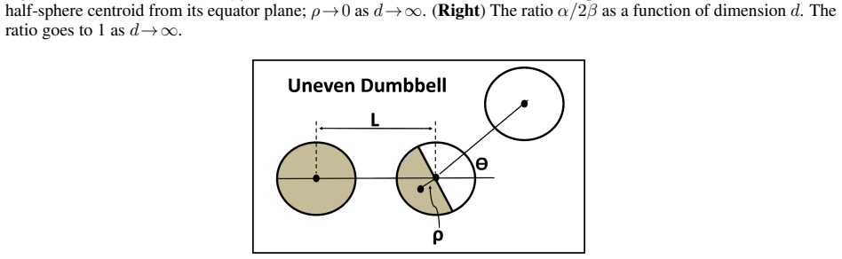
The load-bearing object is the 'ideal cluster': a d-dimensional sphere of radius R and volume V, with all clusters identical, non-overlapping, and dense enough to replace sums by integrals. The argument runs on three closed-form errors—sphere E_s = VR²α, half-sphere E_h = VR²β, and dumbbell E_d = 2E_s + ½VL²—with α = d/(d+2), γ = Γ((d+2)/2)/(√π Γ((d+3)/2)), ρ = Rγ, and β = ½(α − γ²). These feed the interval Nρ²/K < λ < NL²/(2K) for the additive penalty, and also prove that k·E_k has a natural minimum at K. Two deterministic seeding algorithms (Algorithm 1 and Algorithm 2) are introduced to guarantee that, for ideal clusters, the k-means iterations reach the true centroids, so the error formulas genuinely describe the optimized configurations.
What would settle it
Compute both candidate upper bounds from the paper's formulas for, say, d = 2 and L = 2R: the perfect-dumbbell bound λ_d = ½VL² and the uneven-dumbbell bound λ_u = (V/3)(2L² − 4LRγ − R²γ²). Since inequality (B-7) holds with γ = 0.424, λ_u is strictly smaller than λ_d, which refutes the claim that the perfect-dumbbell bound is the tightest upper bound for all dimensions; a reader can verify this arithmetic in a few lines.
Extended reading notes
Core claim
Under the ideal-cluster assumption—clusters are identical, non-overlapping, densely filled d-dimensional spheres—the paper derives exact expressions for the k-means error of a sphere, a half-sphere, and a dumbbell, and uses them to prove that the additive regularized error E_k + λk has its global minimum at the correct number of clusters K exactly when Nρ²/K < λ < NL²/(2K). The lower bound comes from comparing K spheres with K+1 clusters where one sphere splits into two half-spheres; the upper bound comes from comparing K spheres with K−1 clusters where two adjacent spheres merge into a dumbbell. The paper argues that the perfect-dumbbell configuration gives the tightest upper bound in most dimensions, and recommends the midpoint λ ≈ NL²/(4K) as a repeatable choice. For the multiplicative regularizer k·E_k, no such parameter is needed: the same geometric error formulas imply the regularized error is minimized at K for all d ≥ 2 and K ≥ 2.
Load-bearing premise
The upper bound relies on the assumption that when the algorithm has one fewer cluster than the true count, the best achievable configuration is a perfect dumbbell, and that this configuration yields the tightest upper bound in every dimension; the paper's own Appendix B shows this tightness fails for d ≤ 9 when L = 2R.
Editorial extensions
If this is right
- For ideal clusters, a user can set λ by measuring N, the smallest inter-centroid distance L, and the sphere radius R, then pick the midpoint of the interval as a repeatable default.
- The multiplicative regularizer k·E_k requires no hyperparameter at all for ideal clusters, giving a parameter-free baseline for cluster-count selection.
- When additive and multiplicative regularizers disagree, their consensus candidates can be treated as the plausible cluster counts, which the experiments show reduces ambiguity in overlapping or non-spherical data.
- The same interval logic extends to other penalty shapes (logarithmic, power, exponential) by replacing the differences f(K+1)−f(K) and f(K)−f(K−1) in the bounds, as derived in Appendix C.
- The results apply most directly in high dimensions, where cluster overlap is smaller and the ideal-cluster approximation is better.
Reading between the lines
- The claim that the perfect dumbbell gives the tightest upper bound in every dimension is not supported even by the paper's own Appendix B: for L = 2R and d ≤ 9, an uneven dumbbell yields a smaller upper bound, so in those cases Eq. (11) is valid but not tight; a dimension-corrected upper bound would be needed before the interval is called rigorous in low dimensions.
- The midpoint recommendation λ ≈ NL²/(4K) could be tested as a default on non-ideal data with known cluster structure; if it systematically under- or over-counts, the failure mode would point to how strongly the no-overlap assumption is being violated.
- One could extend the analysis to unequal cluster radii or overlapping Gaussian clusters by numerically computing the sphere-split and dumbbell errors instead of the closed forms, retaining the same bound structure with computed quantities.
- The consensus criterion between additive and multiplicative solutions could be formalized as a scoring rule (e.g., counting agreement across many restarts), which would quantize the ambiguity the paper reports qualitatively.
Editorial analysis
A structured set of objections, weighed in public.
Referee Report
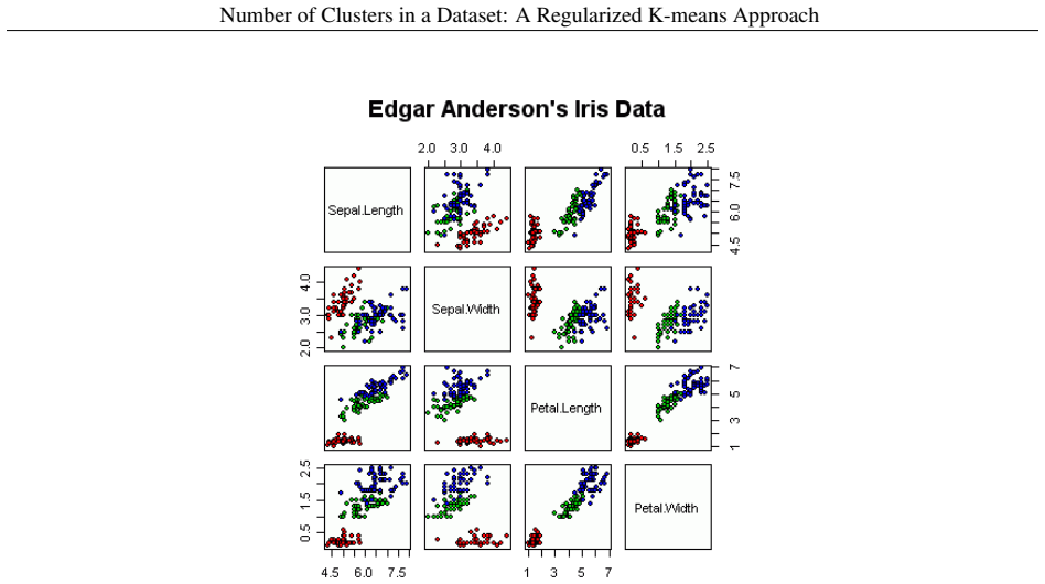
Summary. This paper studies the problem of estimating the number of clusters K in unlabeled data using regularized k-means objectives, specifically E_k^(a) = E_k + lambda k and E_k^(m) = k E_k. Under an "ideal cluster" model (equal, non-overlapping d-dimensional spheres uniformly filled with data points), the authors derive lower and upper bounds for the additive penalty coefficient lambda, stated in Eq. (11) as N rho^2 / K < lambda < N L^2 / (2K), and propose a midpoint rule combined with an assumed-K enumeration procedure. They also analyze the multiplicative regularizer, argue that it has a natural minimum at K for ideal clusters, and present experiments on simulated data, a textured image, and the Iris dataset. The central claim is that Eq. (11) provides rigorous, dimension-uniform bounds on lambda under the ideal-cluster assumption.
Significance. A principled interval for the additive penalty coefficient would address a real practical gap, since lambda is normally chosen ad hoc; the lower-bound derivation from the K versus K+1 comparison is clean, and the geometric treatment in the appendices is mostly self-contained. The multiplicative regularizer is parameter-free and appears empirically more robust, and the consensus idea between additive and multiplicative penalties is sensible. However, the paper's central rigor claim is undercut by its own Appendix B: for L = 2R and d <= 9, the uneven dumbbell gives a strictly tighter upper bound than the perfect dumbbell, so Eq. (11) is not valid for all dimensions as stated. In addition, the proposed method for selecting lambda depends on the unknown values of K and L, which limits its practical use as a principled guideline. If the upper-bound gap is repaired and the practical procedure is clarified, the contribution would be solid; in its present form the main theorem is overstated.
major comments (3)
- [Sec. 4 and Appendix B, Eq. (B-7)] The assertion in Sec. 4 that the perfect dumbbell "yields the tightest bound for all dimensions" is contradicted by the paper's own inequality (B-7). For non-overlapping spheres with L = 2R, inequality (B-7) holds whenever gamma > 0.243, i.e., for dimension d <= 9, and then lambda_u from Eq. (B-6) is strictly smaller than lambda_d from Eq. (B-4). For example, for d = 2, L = 2R, gamma ~= 0.424, lambda_u ~= 1.477 V R^2 while lambda_d = 2 V R^2. A value lambda in (lambda_u, lambda_d) lies inside the interval advertised by Eq. (11) yet makes E^(u)_{K-1} - E_K - lambda < 0, so K is not even a local minimum of the additively regularized error. The defense in Appendix B that lambda_d is dimension-independent and smaller for most dimensions is not a proof of tightness for all dimensions. This is a load-bearing gap in the central result, not a minor caveat; the upper bound in Eq. (11) must be replaced by a bound that is actually valid for the optimal K-1 configuration, or the claim must be restricted accordingly.
- [Sec. 4.1 and Eq. (12)] The proposed procedure requires K and L before lambda can be set, and L is the smallest inter-centroid distance of the unknown true configuration. The "assume K, then check" loop still needs an estimate of L for each assumed K, so the user must either supply external knowledge or estimate L from a K-cluster solution, which biases the test. The paper acknowledges this dependence, but it means that the method is not a fully data-driven principled guideline. Please specify exactly how L is estimated in the experiments and discuss how sensitive the candidate-solution sets are to that estimate.
- [Eq. (10) and abstract] The conditions in Eq. (10) only ensure that E^(a)_K is lower than its immediate neighbors E^(a)_{K-1} and E^(a)_{K+1}. The abstract and Sec. 4 state that the regularized error has its global minimum at K, but no argument excludes the possibility of a lower value at k < K-1 or k > K+1 under the same lambda. If the global claim is intended, a proof is needed; otherwise the text should consistently say "local minimum" rather than "global minimum."
minor comments (4)
- [Throughout] There are several typos in the text and figure captions, including "regularizd" in Sec. 7, "shonw" in Fig. 5, "Muliplicative" and "Clsuters" in Fig. 7, and "aditive" in Fig. 8.
- [Sec. 4 and Sec. 5] The citation "as may also be seen in Fig. 8" for the alpha/(2 beta) ratio is incorrect: Fig. 8 is the 8-dimensional cluster example, while the ratio is plotted in Fig. 13 of Appendix A. The cross-reference should be fixed.
- [Sec. 6.2] The "consensus" criterion between additive and multiplicative candidate solutions is not formally defined. Please state precisely whether it means the intersection of the two candidate sets, and how ties or near-misses are treated.
- [Sec. 3.1 and Sec. 3.2] The algorithms are presented as deterministic, but tie-breaking in the "choose the farthest point" steps is unspecified; for ideal equal spheres with L = 2R, ties can occur, which affects the claim that a distinct cluster is always selected as the initial centroid.
Circularity Check
No derivation-level circularity; one acknowledged fixed-point dependency of lambda on the unknown K keeps the paper at a low circularity score.
-
other
[Sec. 4, Eq. (11); Sec. 4.1]
"Note that λ depends on the correct number of clusters K, the hyper-parameter we want to determine. This introduces another layer of complexity in using k-means with additive penalty."
The interval in Eq. (11) is stated in terms of K (and L, the smallest inter-centroid distance), where K is precisely the quantity the procedure is supposed to determine. Sec. 4.1 then instructs the user to assume a value of K, select λ from the interval computed with that assumed K, run k-means, and check whether the regularized error has a minimum at the assumed K. Thus the test for K being correct uses a λ that was chosen from the hypothesis K itself, making the procedure a fixed-point or self-consistency check rather than an independent estimate of K. The paper explicitly acknowledges this dependency, labels the outputs 'potential solutions,' and does not hide the circularity.
full rationale
The core derivation of Eq. (11) is self-contained geometry: the errors E_{K-1}, E_K, and E_{K+1} are obtained from explicit integrals for spheres, half-spheres, and dumbbells in Appendix A, and the inequalities delta^{(a)}_{K-1,K} > 0 and delta^{(a)}_{K,K+1} < 0 are pure algebraic consequences of those cluster shapes. No parameter is fitted to data, and no load-bearing result is imported from the authors' prior work; the self-citation [22] is background and does not carry the argument. The only circularity-adjacent element is that the lambda interval depends on K and L, the very quantities one wants to infer, and Sec. 4.1 uses lambda obtained from an assumed K to test whether that K is a minimum. The paper acknowledges this twice, and the procedure is explicitly a search for 'potential solutions' rather than a one-shot prediction. In addition, Appendix B's inequality (B-7) shows that for d <= 9 and L = 2R the uneven dumbbell gives a smaller upper bound than the perfect dumbbell, which contradicts Sec. 4's blanket claim that the perfect dumbbell yields the tightest bound for all dimensions. That is a correctness gap in the stated rigor of the upper bound, but it is not circularity and does not raise the circularity score. Overall, the mathematical derivation is independent and self-contained; the acknowledged K-dependence of lambda warrants only a low circularity score of 2.
Assumptions & free parameters
free parameters (2)
- Midpoint rule for lambda =
lambda ~ N(rho^2 + 0.5 L^2)/(2K) ~ N L^2/(4K)
- Outlier culling threshold =
not specified
assumptions (4)
- domain assumption Ideal clusters are d-dimensional spheres of equal radius, non-overlapping, with no outliers, and dense enough that the number of points per cluster equals the sphere volume V.
- ad hoc to paper For k = K-1, the optimal clustering is either one perfect dumbbell plus K-2 spheres, or two uneven dumbbells plus K-3 spheres, and the perfect dumbbell yields the tightest upper bound for all dimensions.
- domain assumption The number of data points per ideal cluster is approximated by the sphere volume V, so N approx K V.
- domain assumption Algorithms 1 and 2 are provably optimal for ideal clusters when k = K.
Cite this review
Pith. "Pith review of Number of Clusters in a Dataset: A Regularized K-means Approach." pith.science (2026). https://pith.science/paper/M6MPXTKL
@misc{pith2026250522991,
  author       = {Pith},
  title        = {Pith review of: Number of Clusters in a Dataset: A Regularized K-means Approach},
  year         = {2026},
  howpublished = {\url{https://pith.science/paper/M6MPXTKL}},
  note         = {Machine review of arXiv:2505.22991}
}
abstract
Finding the number of meaningful clusters in an unlabeled dataset is important in many applications. Regularized k-means algorithm is a possible approach frequently used to find the correct number of distinct clusters in datasets. The most common formulation of the regularization function is the additive linear term $\lambda k$, where $k$ is the number of clusters and $\lambda$ a positive coefficient. Currently, there are no principled guidelines for setting a value for the critical hyperparameter $\lambda$. In this paper, we derive rigorous bounds for $\lambda$ assuming clusters are {\em ideal}. Ideal clusters (defined as $d$-dimensional spheres with identical radii) are close proxies for k-means clusters ($d$-dimensional spherically symmetric distributions with identical standard deviations). Experiments show that the k-means algorithm with additive regularizer often yields multiple solutions. Thus, we also analyze k-means algorithm with multiplicative regularizer. The consensus among k-means solutions with additive and multiplicative regularizations reduces the ambiguity of multiple solutions in certain cases. We also present selected experiments that demonstrate performance of the regularized k-means algorithms as clusters deviate from the ideal assumption.
Figures


Figures from the paper (11 more)




Reference graph
Works this paper leans on
-
[22]
B. Kamgar-Parsi and B. Kamgar-Parsi. Penalized K-Means Algorithms for Finding the Number of Clusters. Proc. 2020 International Conference on Pattern Recognition (ICPR 2020), Milan, Italy, Jan. 10-15, 2021, pp. 969-974
work page 2020
-
[1]
S. Ahmadian, A. Norouzi-Fard, O. Svensson, J. Ward. Better Guarantees for k-Means and Euclidean k-Median by Primal-Dual Algorithms. Proc. FOCS, pp. 61-72, 2017
work page 2017
-
[2]
Recovering the number of clusters in data sets with noise features using feature rescaling factors
R.C. de Amorim and C. Henning. Recovering the number of clusters in data sets with noise features using feature rescaling factors. arXiv:1602.06989v1, Feb. 2016
work page Pith review arXiv 2016
- [3]
-
[4]
D. Arthur and S. Vassilvitskii. k-means++: The Advantages of Careful Seeding. Proc. Annual ACM-SIAM Sympo- sium on Discrete Algorithms (SODA), pp. 1027-1035, 2007
work page 2007
- [5]
-
[6]
Recombinator-k-means: An evolutionary algorithm that exploits k-means++ for recombination
C. Baldassi. Recombinator-k-means: Enhancing k-means++ by seeding from pools of previous runs. arXiv:1905.00531v1, May 2019
work page Pith review arXiv 1905
-
[7]
A. Blum, J. Hopcroft, and R. Kannan. Foundations of Data Science, Cambridge University Press, 2020
work page 2020
Show all 40 references
-
[8]
Bozdogan
H. Bozdogan. Model selection and Akaike’s information criterion (AIC): the general theory and its analytical extensions. Psychometrika, 52(3):345–370, 1987
1987
-
[9]
P.J.A. Cock. https://warwick.ac.uk/fac/sci/moac/people/students /peter_cock/r/iris_plots/
-
[10]
R.O. Duda, P. E. Hart, and D.G. Stork. Pattern Classification. Wiley, 2003
2003
-
[11]
A. Fischer. On the number of groups in clustering. Statistics and Probability Letters, 81:1771–1781, 2011
2011
-
[12]
Frank and A
A. Frank and A. Asuncion. UCI Machine Learning Repository. University of California, Irvine, School of Information and Computer Sciences, 2010. http://archive.ics.uci.edu/ml
2010
-
[13]
Franti and S
P. Franti and S. Sieranoja. How much can k-means be improved by using better initialization and repeats? Pattern Recognition, 93(9):95-112, 2019
2019
-
[14]
Fu and P.O
W. Fu and P.O. Perry. Estimating the number of clusters using cross-validation. arXiv:1702.02658v1, Feb. 2017
2017 arXiv
-
[15]
Fujita, D.Y
A. Fujita, D.Y . Takahashi, and A.G. Patriota. A non-parametric method to estimate the number of clusters. Computational Statistics and Data Analysis, 73:27-39, 2014
2014
-
[16]
Gersho and R.M
A. Gersho and R.M. Gray. Vector Quantization and Signal Compression. Kluwer Academic Publishers, 1992
1992
-
[17]
Gradshteyn and I.M
I.S. Gradshteyn and I.M. Ryzhik. Table of Integrals, Series, and Products, Academic Press, 4th edition, p. 369, 1965
1965
-
[18]
Jain and R.C
A.K. Jain and R.C. Dubes. Algorithms for Clustering Data. Prentice-Hall, 1988
1988
-
[19]
A.K. Jain. Data clustering: 50 years beyond K-means. Pattern Recognition Letters, 31(8):651-666, 2010
2010
-
[20]
Kamgar-Parsi, J.A
B. Kamgar-Parsi, J.A. Gualtieri, J.E. Devaney, and B. Kamgar-Parsi. Clustering with neural networks.Biological Cybernetics, 63(3):201-208, 1990
1990
-
[21]
Kamgar-Parsi and B
B. Kamgar-Parsi and B. Kamgar-Parsi. Dynamical Stability and Parameter Selection in Neural Optimization.Proc. International Joint Conference on Neural Networks, 4:566-571, 1992
1992
-
[23]
Kanungo, D.M
T. Kanungo, D.M. Mount, N.S. Netanyahu, C.D. Piatko, R. Silverman, and A.Y . Wu. An Efficient k-Means Clustering Algorithm: Analysis and Implementation. IEEE Trans. Pattern Analysis and Machine Intelligence , 24(7):881-892, 2002
2002
-
[24]
Krzanowski and Y .T
W.J. Krzanowski and Y .T. Lai. A criterion for determining the number of clusters in a data set. Biometrics, 44:23–34, 1988
1988
-
[25]
Kulis and M.I
B. Kulis and M.I. Jordan. Revisiting k-means: New Algorithms via Bayesian Nonparametrics. Proc. International Conference on Machine Learning (ICML), Edinburgh, UK, 2012
2012
-
[26]
W. Li, E.K. Ryu, S. Osher, W. Yin, and W. Gangbo. A parallel method for earth mover’s distance.UCLA Comput. Appl. Math. Pub. (CAM) Rep., 17-12, 2017
2017
-
[27]
Linde, A
Y . Linde, A. Buzo, and R. Gray. An Algorithm for Vector Quantizer Design. IEEE Trans. Communications, 28:84-95, 1980. 14 Number of Clusters in a Dataset: A Regularized K-means Approach
1980
-
[28]
S. P. Lloyd. Least squares quantization in PCM. IEEE Trans. Information Theory, 28(2):129-137, 1982. Appeared first in a 1956 AT&T Bell Labs memorandum
1982
-
[29]
Manning, P
C.D. Manning, P. Raghavan, and H. Schutze.Introduction to Information retrieval. Cambridge University Press, 2008
2008
-
[30]
K.P. Murphy. Machine Learning: A Probabilistic Perspective. MIT Press, 2012
2012
-
[31]
K. Rose, E. Gurewitz, and G.C. Fox. Vector quantization by deterministic annealing.IEEE Trans. Information Theory, 38(4):1249-1257, 1992
1992
-
[32]
Rousseeuw
P.J. Rousseeuw. Silhouettes: A graphical aid to the interpretation and validation of cluster analysis.Journal of Computational and Applied Mathematics, 20:53-65, 1987
1987
-
[33]
J.W. Sammon. A Nonlinear Mapping for Data Structure Analysis. IEEE Trans. Computers, 18(5):401–409, 1969
1969
-
[34]
G. Schwarz. Estimating the dimension of a model. The Annals of Statistics, 6(2):461–464, 1978
1978
-
[35]
Sugar and G.M
C.A. Sugar and G.M. James. Finding the number of clusters in a dataset: an information-theoretic approach. Journal of the American Statistical Association, 98(463):750-763, 2003
2003
-
[36]
Szczypi´nski, M
P. Szczypi´nski, M. Strzelecki, and A. Materka. MaZda A Software for Texture Analysis. Proc. Int’l Symp. on Information Technology Convergence, ISITC 2007
2007
-
[37]
Tibshirani, G
R. Tibshirani, G. Walther, and T. Hastie. Estimating the number of clusters in a data set via the gap statistic. Journal of the Royal Statistical Society, 63(2):411-423, 2001
2001
-
[38]
Vidal, Y
R. Vidal, Y . Ma, and S. Sastry.Generalized Principal Component Analysis, Springer-Verlag, 2016
2016
-
[39]
https://en.wikipedia.org/wiki/Determining_the_number_of_ clusters_in_a_data_set. 15 Number of Clusters in a Dataset: A Regularized K-means Approach Appendix A: Single-Cluster Variances In this Appendix, we calculate the volume of a sphere in then-dimensional Euclidean space, a...
-
[40]
(A-4) With repeated use of (A-3), Eq
= (2n)!√π 4nn! . (A-4) With repeated use of (A-3), Eq. (A-2) simplifies to: V = π n 2 Γ(n + 2 2 ) Rn. (A-5) The within-cluster variance, or clustering error, for then-dimensional sphere is given by: Es = ∫ sphere dV ‖ x− c‖2, (A-6) and may be expressed in the spherical coordina...
Reviewed August 7, 2026 · model on record in the stance chip above.
Discussion (0). Sign in to comment.